ทัวร์ชมความน่าจะเป็นของ TensorFlow

ดูบน TensorFlow.org

ทำงานใน Google Colab

ดูแหล่งที่มาบน GitHub

ดาวน์โหลดโน๊ตบุ๊ค

ใน Colab นี้ เราจะสำรวจคุณลักษณะพื้นฐานบางอย่างของความน่าจะเป็นของ TensorFlow

การพึ่งพาและข้อกำหนดเบื้องต้น

นำเข้า

from pprint import pprint
import matplotlib.pyplot as plt
import numpy as np
import seaborn as sns

import tensorflow.compat.v2 as tf
tf.enable_v2_behavior()

import tensorflow_probability as tfp

sns.reset_defaults()
sns.set_context(context='talk',font_scale=0.7)
plt.rcParams['image.cmap'] = 'viridis'

%matplotlib inline

tfd = tfp.distributions
tfb = tfp.bijectors

ยูทิลิตี้

def print_subclasses_from_module(module, base_class, maxwidth=80):
  import functools, inspect, sys
  subclasses = [name for name, obj in inspect.getmembers(module)
                if inspect.isclass(obj) and issubclass(obj, base_class)]
  def red(acc, x):
    if not acc or len(acc[-1]) + len(x) + 2 > maxwidth:
      acc.append(x)
    else:
      acc[-1] += ", " + x
    return acc
  print('\n'.join(functools.reduce(red, subclasses, [])))

เค้าร่าง

• TensorFlow
• ความน่าจะเป็นของเทนเซอร์โฟล
  • การกระจาย
  • Bijectors
  • MCMC
  • ...และอื่น ๆ!

คำนำ: TensorFlow

TensorFlow เป็นห้องสมุดคอมพิวเตอร์ทางวิทยาศาสตร์

รองรับ

• การคำนวณทางคณิตศาสตร์มากมาย
• การคำนวณ vectorized ที่มีประสิทธิภาพ
• การเร่งฮาร์ดแวร์อย่างง่าย
• การแยกความแตกต่างอัตโนมัติ

เวกเตอร์

• Vectorization ทำให้สิ่งต่าง ๆ รวดเร็ว!
• นอกจากนี้ยังหมายความว่าเราคิดมากเกี่ยวกับรูปร่าง

mats = tf.random.uniform(shape=[1000, 10, 10])
vecs = tf.random.uniform(shape=[1000, 10, 1])

def for_loop_solve():
  return np.array(
    [tf.linalg.solve(mats[i, ...], vecs[i, ...]) for i in range(1000)])

def vectorized_solve():
  return tf.linalg.solve(mats, vecs)

# Vectorization for the win!
%timeit for_loop_solve()
%timeit vectorized_solve()

1 loops, best of 3: 2 s per loop
1000 loops, best of 3: 653 µs per loop

การเร่งฮาร์ดแวร์

# Code can run seamlessly on a GPU, just change Colab runtime type
# in the 'Runtime' menu.
if tf.test.gpu_device_name() == '/device:GPU:0':
  print("Using a GPU")
else:
  print("Using a CPU")

Using a CPU

การแยกความแตกต่างอัตโนมัติ

a = tf.constant(np.pi)
b = tf.constant(np.e)
with tf.GradientTape() as tape:
  tape.watch([a, b])
  c = .5 * (a**2 + b**2)
grads = tape.gradient(c, [a, b])
print(grads[0])
print(grads[1])

tf.Tensor(3.1415927, shape=(), dtype=float32)
tf.Tensor(2.7182817, shape=(), dtype=float32)

ความน่าจะเป็นของเทนเซอร์โฟล

ความน่าจะเป็นของ TensorFlow เป็นห้องสมุดสำหรับการให้เหตุผลเชิงความน่าจะเป็นและการวิเคราะห์ทางสถิติใน TensorFlow

เราสนับสนุนการสร้างแบบจำลองการอนุมานและการวิจารณ์ผ่านองค์ประกอบของส่วนประกอบแบบแยกส่วนระดับต่ำ

หน่วยการสร้างระดับต่ำ

• การกระจาย
• Bijectors

โครงสร้างระดับสูง (เอ้อ)

• Markov chain มอนติคาร์โล
• ชั้นความน่าจะเป็น
• อนุกรมเวลาโครงสร้าง
• แบบจำลองเชิงเส้นทั่วไป
• เครื่องมือเพิ่มประสิทธิภาพ

การกระจาย

tfp.distributions.Distribution เป็นชั้นที่มีสองวิธีหลัก: sample และ log_prob

TFP มีการแจกแจงมากมาย!

print_subclasses_from_module(tfp.distributions, tfp.distributions.Distribution)

Autoregressive, BatchReshape, Bates, Bernoulli, Beta, BetaBinomial, Binomial
Blockwise, Categorical, Cauchy, Chi, Chi2, CholeskyLKJ, ContinuousBernoulli
Deterministic, Dirichlet, DirichletMultinomial, Distribution, DoublesidedMaxwell
Empirical, ExpGamma, ExpRelaxedOneHotCategorical, Exponential, FiniteDiscrete
Gamma, GammaGamma, GaussianProcess, GaussianProcessRegressionModel
GeneralizedNormal, GeneralizedPareto, Geometric, Gumbel, HalfCauchy, HalfNormal
HalfStudentT, HiddenMarkovModel, Horseshoe, Independent, InverseGamma
InverseGaussian, JohnsonSU, JointDistribution, JointDistributionCoroutine
JointDistributionCoroutineAutoBatched, JointDistributionNamed
JointDistributionNamedAutoBatched, JointDistributionSequential
JointDistributionSequentialAutoBatched, Kumaraswamy, LKJ, Laplace
LinearGaussianStateSpaceModel, LogLogistic, LogNormal, Logistic, LogitNormal
Mixture, MixtureSameFamily, Moyal, Multinomial, MultivariateNormalDiag
MultivariateNormalDiagPlusLowRank, MultivariateNormalFullCovariance
MultivariateNormalLinearOperator, MultivariateNormalTriL
MultivariateStudentTLinearOperator, NegativeBinomial, Normal, OneHotCategorical
OrderedLogistic, PERT, Pareto, PixelCNN, PlackettLuce, Poisson
PoissonLogNormalQuadratureCompound, PowerSpherical, ProbitBernoulli
QuantizedDistribution, RelaxedBernoulli, RelaxedOneHotCategorical, Sample
SinhArcsinh, SphericalUniform, StudentT, StudentTProcess
TransformedDistribution, Triangular, TruncatedCauchy, TruncatedNormal, Uniform
VariationalGaussianProcess, VectorDeterministic, VonMises
VonMisesFisher, Weibull, WishartLinearOperator, WishartTriL, Zipf

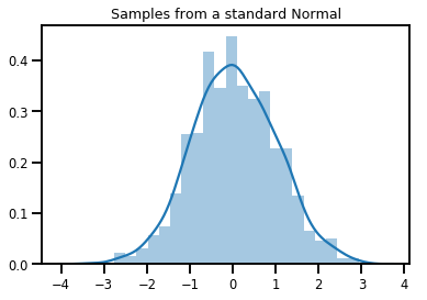
เกลาตัวแปรที่เรียบง่าย Distribution

# A standard normal
normal = tfd.Normal(loc=0., scale=1.)
print(normal)

tfp.distributions.Normal("Normal", batch_shape=[], event_shape=[], dtype=float32)

# Plot 1000 samples from a standard normal
samples = normal.sample(1000)
sns.distplot(samples)
plt.title("Samples from a standard Normal")
plt.show()

# Compute the log_prob of a point in the event space of `normal`
normal.log_prob(0.)

<tf.Tensor: shape=(), dtype=float32, numpy=-0.9189385>

# Compute the log_prob of a few points
normal.log_prob([-1., 0., 1.])

<tf.Tensor: shape=(3,), dtype=float32, numpy=array([-1.4189385, -0.9189385, -1.4189385], dtype=float32)>

การกระจายและรูปร่าง

Numpy ndarrays และ TensorFlow Tensors มีรูปร่าง

TensorFlow ความน่าจะเป็น Distributions มีความหมายรูปร่าง - รูปทรงพาร์ทิชันที่เราเป็นชิ้นที่แตกต่างกันความหมายแม้ว่าก้อนเดียวกันของหน่วยความจำ ( Tensor / ndarray ) ใช้สำหรับทุกอย่างทั้ง

• รูปร่าง Batch หมายถึงคอลเลกชันของ Distribution s กับพารามิเตอร์ที่แตกต่างกัน
• รูปร่างเหตุการณ์หมายถึงรูปร่างของกลุ่มตัวอย่างจาก Distribution

เราใส่รูปร่างชุดที่ "ซ้าย" และรูปร่างเหตุการณ์ที่ "ขวา" เสมอ

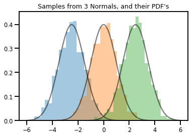
ชุดของสเกลาตัวแปร Distributions

แบทช์เป็นเหมือนการแจกแจงแบบ "เวกเตอร์": อินสแตนซ์อิสระที่มีการคำนวณแบบขนาน

# Create a batch of 3 normals, and plot 1000 samples from each
normals = tfd.Normal([-2.5, 0., 2.5], 1.)  # The scale parameter broadacasts!
print("Batch shape:", normals.batch_shape)
print("Event shape:", normals.event_shape)

Batch shape: (3,)
Event shape: ()

# Samples' shapes go on the left!
samples = normals.sample(1000)
print("Shape of samples:", samples.shape)

Shape of samples: (1000, 3)

# Sample shapes can themselves be more complicated
print("Shape of samples:", normals.sample([10, 10, 10]).shape)

Shape of samples: (10, 10, 10, 3)

# A batch of normals gives a batch of log_probs.
print(normals.log_prob([-2.5, 0., 2.5]))

tf.Tensor([-0.9189385 -0.9189385 -0.9189385], shape=(3,), dtype=float32)

# The computation broadcasts, so a batch of normals applied to a scalar
# also gives a batch of log_probs.
print(normals.log_prob(0.))

tf.Tensor([-4.0439386 -0.9189385 -4.0439386], shape=(3,), dtype=float32)

# Normal numpy-like broadcasting rules apply!
xs = np.linspace(-6, 6, 200)
try:
  normals.log_prob(xs)
except Exception as e:
  print("TFP error:", e.message)

TFP error: Incompatible shapes: [200] vs. [3] [Op:SquaredDifference]

# That fails for the same reason this does:
try:
  np.zeros(200) + np.zeros(3)
except Exception as e:
  print("Numpy error:", e)

Numpy error: operands could not be broadcast together with shapes (200,) (3,)

# But this would work:
a = np.zeros([200, 1]) + np.zeros(3)
print("Broadcast shape:", a.shape)

Broadcast shape: (200, 3)

# And so will this!
xs = np.linspace(-6, 6, 200)[..., np.newaxis]
# => shape = [200, 1]

lps = normals.log_prob(xs)
print("Broadcast log_prob shape:", lps.shape)

Broadcast log_prob shape: (200, 3)

# Summarizing visually
for i in range(3):
  sns.distplot(samples[:, i], kde=False, norm_hist=True)
plt.plot(np.tile(xs, 3), normals.prob(xs), c='k', alpha=.5)
plt.title("Samples from 3 Normals, and their PDF's")
plt.show()

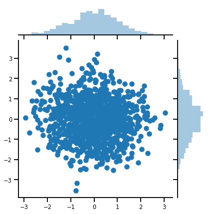
เวกเตอร์ตัวแปร Distribution

mvn = tfd.MultivariateNormalDiag(loc=[0., 0.], scale_diag = [1., 1.])
print("Batch shape:", mvn.batch_shape)
print("Event shape:", mvn.event_shape)

Batch shape: ()
Event shape: (2,)

samples = mvn.sample(1000)
print("Samples shape:", samples.shape)

Samples shape: (1000, 2)

g = sns.jointplot(samples[:, 0], samples[:, 1], kind='scatter')
plt.show()

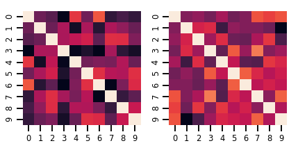
เมทริกซ์ตัวแปร Distribution

lkj = tfd.LKJ(dimension=10, concentration=[1.5, 3.0])
print("Batch shape: ", lkj.batch_shape)
print("Event shape: ", lkj.event_shape)

Batch shape:  (2,)
Event shape:  (10, 10)

samples = lkj.sample()
print("Samples shape: ", samples.shape)

Samples shape:  (2, 10, 10)

fig, axes = plt.subplots(nrows=1, ncols=2, figsize=(6, 3))
sns.heatmap(samples[0, ...], ax=axes[0], cbar=False)
sns.heatmap(samples[1, ...], ax=axes[1], cbar=False)
fig.tight_layout()
plt.show()

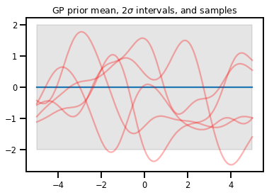
กระบวนการเกาส์เซียน

kernel = tfp.math.psd_kernels.ExponentiatedQuadratic()
xs = np.linspace(-5., 5., 200).reshape([-1, 1])
gp = tfd.GaussianProcess(kernel, index_points=xs)
print("Batch shape:", gp.batch_shape)
print("Event shape:", gp.event_shape)

Batch shape: ()
Event shape: (200,)

upper, lower = gp.mean() + [2 * gp.stddev(), -2 * gp.stddev()]
plt.plot(xs, gp.mean())
plt.fill_between(xs[..., 0], upper, lower, color='k', alpha=.1)
for _ in range(5):
  plt.plot(xs, gp.sample(), c='r', alpha=.3)
plt.title(r"GP prior mean, $2\sigma$ intervals, and samples")
plt.show()

#    *** Bonus question ***
# Why do so many of these functions lie outside the 95% intervals?

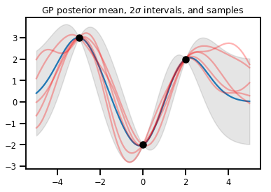
GP Regression

# Suppose we have some observed data
obs_x = [[-3.], [0.], [2.]]  # Shape 3x1 (3 1-D vectors)
obs_y = [3., -2., 2.]        # Shape 3   (3 scalars)

gprm = tfd.GaussianProcessRegressionModel(kernel, xs, obs_x, obs_y)

upper, lower = gprm.mean() + [2 * gprm.stddev(), -2 * gprm.stddev()]
plt.plot(xs, gprm.mean())
plt.fill_between(xs[..., 0], upper, lower, color='k', alpha=.1)
for _ in range(5):
  plt.plot(xs, gprm.sample(), c='r', alpha=.3)
plt.scatter(obs_x, obs_y, c='k', zorder=3)
plt.title(r"GP posterior mean, $2\sigma$ intervals, and samples")
plt.show()

Bijectors

Bijectors เป็นตัวแทนของ (ส่วนใหญ่) พลิกกลับ, ฟังก์ชั่นที่ราบรื่น สามารถใช้ในการแปลงการแจกแจง โดยคงความสามารถในการเก็บตัวอย่างและคำนวณ log_probs พวกเขาสามารถอยู่ใน tfp.bijectors โมดูล

bijector แต่ละตัวดำเนินการอย่างน้อย 3 วิธี:

• forward ,
• inverse และ
• (อย่างน้อย) หนึ่งใน forward_log_det_jacobian และ inverse_log_det_jacobian

ด้วยส่วนผสมเหล่านี้ เราสามารถเปลี่ยนรูปแบบการจัดจำหน่ายและยังคงได้รับตัวอย่างและบันทึกปัญหาจากผลลัพธ์!

ในวิชาคณิตศาสตร์ค่อนข้างเลอะเทอะ

• \(X\) เป็นตัวแปรสุ่มที่มีรูปแบบไฟล์ PDF \(p(x)\)
• \(g\) เป็นเรียบฟังก์ชั่นกลับด้านบนพื้นที่ว่างของ \(X\)'s
• \(Y = g(X)\) เป็นใหม่เปลี่ยนตัวแปรสุ่ม
• \(p(Y=y) = p(X=g^{-1}(y)) \cdot |\nabla g^{-1}(y)|\)

เก็บเอาไว้

Bijectors ยังแคชการคำนวณไปข้างหน้าและย้อนกลับ และ log-det-Jacobians ซึ่งช่วยให้เราบันทึกการดำเนินการซ้ำที่อาจมีราคาแพงมากได้!

print_subclasses_from_module(tfp.bijectors, tfp.bijectors.Bijector)

AbsoluteValue, Affine, AffineLinearOperator, AffineScalar, BatchNormalization
Bijector, Blockwise, Chain, CholeskyOuterProduct, CholeskyToInvCholesky
CorrelationCholesky, Cumsum, DiscreteCosineTransform, Exp, Expm1, FFJORD
FillScaleTriL, FillTriangular, FrechetCDF, GeneralizedExtremeValueCDF
GeneralizedPareto, GompertzCDF, GumbelCDF, Identity, Inline, Invert
IteratedSigmoidCentered, KumaraswamyCDF, LambertWTail, Log, Log1p
MaskedAutoregressiveFlow, MatrixInverseTriL, MatvecLU, MoyalCDF, NormalCDF
Ordered, Pad, Permute, PowerTransform, RationalQuadraticSpline, RayleighCDF
RealNVP, Reciprocal, Reshape, Scale, ScaleMatvecDiag, ScaleMatvecLU
ScaleMatvecLinearOperator, ScaleMatvecTriL, ScaleTriL, Shift, ShiftedGompertzCDF
Sigmoid, Sinh, SinhArcsinh, SoftClip, Softfloor, SoftmaxCentered, Softplus
Softsign, Split, Square, Tanh, TransformDiagonal, Transpose, WeibullCDF

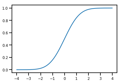
ง่าย Bijector

normal_cdf = tfp.bijectors.NormalCDF()
xs = np.linspace(-4., 4., 200)
plt.plot(xs, normal_cdf.forward(xs))
plt.show()

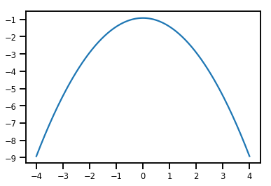
plt.plot(xs, normal_cdf.forward_log_det_jacobian(xs, event_ndims=0))
plt.show()

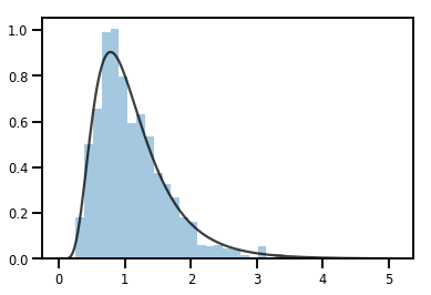
Bijector ปรับเปลี่ยน Distribution

exp_bijector = tfp.bijectors.Exp()
log_normal = exp_bijector(tfd.Normal(0., .5))

samples = log_normal.sample(1000)
xs = np.linspace(1e-10, np.max(samples), 200)
sns.distplot(samples, norm_hist=True, kde=False)
plt.plot(xs, log_normal.prob(xs), c='k', alpha=.75)
plt.show()

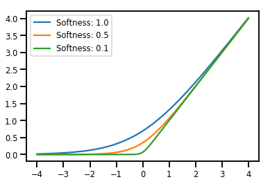
เครื่องผสม Bijectors

# Create a batch of bijectors of shape [3,]
softplus = tfp.bijectors.Softplus(
  hinge_softness=[1., .5, .1])
print("Hinge softness shape:", softplus.hinge_softness.shape)

Hinge softness shape: (3,)

# For broadcasting, we want this to be shape [200, 1]
xs = np.linspace(-4., 4., 200)[..., np.newaxis]
ys = softplus.forward(xs)
print("Forward shape:", ys.shape)

Forward shape: (200, 3)

# Visualization
lines = plt.plot(np.tile(xs, 3), ys)
for line, hs in zip(lines, softplus.hinge_softness):
  line.set_label("Softness: %1.1f" % hs)
plt.legend()
plt.show()

เก็บเอาไว้

# This bijector represents a matrix outer product on the forward pass,
# and a cholesky decomposition on the inverse pass. The latter costs O(N^3)!
bij = tfb.CholeskyOuterProduct()

size = 2500
# Make a big, lower-triangular matrix
big_lower_triangular = tf.eye(size)
# Squaring it gives us a positive-definite matrix
big_positive_definite = bij.forward(big_lower_triangular)

# Caching for the win!
%timeit bij.inverse(big_positive_definite)
%timeit tf.linalg.cholesky(big_positive_definite)

10000 loops, best of 3: 114 µs per loop
1 loops, best of 3: 208 ms per loop

MCMC

TFP ได้สร้างการรองรับอัลกอริธึมของ Markov chain Monte Carlo มาตรฐานบางตัว รวมถึง Hamiltonian Monte Carlo

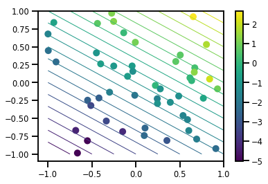
สร้างชุดข้อมูล

# Generate some data
def f(x, w):
  # Pad x with 1's so we can add bias via matmul
  x = tf.pad(x, [[1, 0], [0, 0]], constant_values=1)
  linop = tf.linalg.LinearOperatorFullMatrix(w[..., np.newaxis])
  result = linop.matmul(x, adjoint=True)
  return result[..., 0, :]

num_features = 2
num_examples = 50
noise_scale = .5
true_w = np.array([-1., 2., 3.])

xs = np.random.uniform(-1., 1., [num_features, num_examples])
ys = f(xs, true_w) + np.random.normal(0., noise_scale, size=num_examples)

# Visualize the data set
plt.scatter(*xs, c=ys, s=100, linewidths=0)

grid = np.meshgrid(*([np.linspace(-1, 1, 100)] * 2))
xs_grid = np.stack(grid, axis=0)
fs_grid = f(xs_grid.reshape([num_features, -1]), true_w)
fs_grid = np.reshape(fs_grid, [100, 100])
plt.colorbar()
plt.contour(xs_grid[0, ...], xs_grid[1, ...], fs_grid, 20, linewidths=1)
plt.show()

กำหนดฟังก์ชัน log-prob ร่วมกันของเรา

หลัง unnormalized เป็นผลมาจากการปิดมากกว่าข้อมูลในรูปแบบที่ ประยุกต์ใช้บางส่วน ของ prob บันทึกร่วมกัน

# Define the joint_log_prob function, and our unnormalized posterior.
def joint_log_prob(w, x, y):
  # Our model in maths is
  #   w ~ MVN([0, 0, 0], diag([1, 1, 1]))
  #   y_i ~ Normal(w @ x_i, noise_scale),  i=1..N

  rv_w = tfd.MultivariateNormalDiag(
    loc=np.zeros(num_features + 1),
    scale_diag=np.ones(num_features + 1))

  rv_y = tfd.Normal(f(x, w), noise_scale)
  return (rv_w.log_prob(w) +
          tf.reduce_sum(rv_y.log_prob(y), axis=-1))

# Create our unnormalized target density by currying x and y from the joint.
def unnormalized_posterior(w):
  return joint_log_prob(w, xs, ys)

สร้าง HMC TransitionKernel และเรียก sample_chain

# Create an HMC TransitionKernel
hmc_kernel = tfp.mcmc.HamiltonianMonteCarlo(
  target_log_prob_fn=unnormalized_posterior,
  step_size=np.float64(.1),
  num_leapfrog_steps=2)

# We wrap sample_chain in tf.function, telling TF to precompile a reusable
# computation graph, which will dramatically improve performance.
@tf.function
def run_chain(initial_state, num_results=1000, num_burnin_steps=500):
  return tfp.mcmc.sample_chain(
    num_results=num_results,
    num_burnin_steps=num_burnin_steps,
    current_state=initial_state,
    kernel=hmc_kernel,
    trace_fn=lambda current_state, kernel_results: kernel_results)

initial_state = np.zeros(num_features + 1)
samples, kernel_results = run_chain(initial_state)
print("Acceptance rate:", kernel_results.is_accepted.numpy().mean())

Acceptance rate: 0.915

ที่ไม่ดี! เราต้องการอัตราการยอมรับที่ใกล้กว่า .65

(ดู "ที่เหมาะสมที่สุดสำหรับการปรับขนาดต่างๆ Metropolis-เฮสติ้งส์อัลกอริทึม" โรเบิร์ตและโรเซนธาล, 2001)

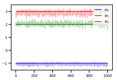
ขนาดขั้นตอนที่ปรับเปลี่ยนได้

เราสามารถตัด HMC TransitionKernel เราใน SimpleStepSizeAdaptation "อภิเคอร์เนล" ซึ่งจะนำไปใช้บางส่วน (แก้ปัญหาค่อนข้างง่าย) ตรรกะในการปรับขนาดขั้นตอน HMC ระหว่าง Burnin เราจัดสรรเบิร์นอิน 80% เพื่อปรับขนาดขั้นตอน แล้วปล่อยให้ 20% ที่เหลือไปผสมกัน

# Apply a simple step size adaptation during burnin
@tf.function
def run_chain(initial_state, num_results=1000, num_burnin_steps=500):
  adaptive_kernel = tfp.mcmc.SimpleStepSizeAdaptation(
      hmc_kernel,
      num_adaptation_steps=int(.8 * num_burnin_steps),
      target_accept_prob=np.float64(.65))

  return tfp.mcmc.sample_chain(
    num_results=num_results,
    num_burnin_steps=num_burnin_steps,
    current_state=initial_state,
    kernel=adaptive_kernel,
    trace_fn=lambda cs, kr: kr)

samples, kernel_results = run_chain(
  initial_state=np.zeros(num_features+1))
print("Acceptance rate:", kernel_results.inner_results.is_accepted.numpy().mean())

Acceptance rate: 0.634

# Trace plots
colors = ['b', 'g', 'r']
for i in range(3):
  plt.plot(samples[:, i], c=colors[i], alpha=.3)
  plt.hlines(true_w[i], 0, 1000, zorder=4, color=colors[i], label="$w_{}$".format(i))
plt.legend(loc='upper right')
plt.show()

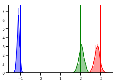
# Histogram of samples
for i in range(3):
  sns.distplot(samples[:, i], color=colors[i])
ymax = plt.ylim()[1]
for i in range(3):
  plt.vlines(true_w[i], 0, ymax, color=colors[i])
plt.ylim(0, ymax)
plt.show()

การวินิจฉัย

พล็อตการติดตามนั้นดี แต่การวินิจฉัยนั้นดีกว่า!

ก่อนอื่นเราต้องรันหลายเชน นี้เป็นง่ายๆเป็นให้ชุดของ initial_state เทนเซอร์

# Instead of a single set of initial w's, we create a batch of 8.
num_chains = 8
initial_state = np.zeros([num_chains, num_features + 1])

chains, kernel_results = run_chain(initial_state)

r_hat = tfp.mcmc.potential_scale_reduction(chains)
print("Acceptance rate:", kernel_results.inner_results.is_accepted.numpy().mean())
print("R-hat diagnostic (per latent variable):", r_hat.numpy())

Acceptance rate: 0.59175
R-hat diagnostic (per latent variable): [0.99998395 0.99932185 0.9997064 ]

สุ่มตัวอย่างระดับเสียงรบกวน

# Define the joint_log_prob function, and our unnormalized posterior.
def joint_log_prob(w, sigma, x, y):
  # Our model in maths is
  #   w ~ MVN([0, 0, 0], diag([1, 1, 1]))
  #   y_i ~ Normal(w @ x_i, noise_scale),  i=1..N

  rv_w = tfd.MultivariateNormalDiag(
    loc=np.zeros(num_features + 1),
    scale_diag=np.ones(num_features + 1))

  rv_sigma = tfd.LogNormal(np.float64(1.), np.float64(5.))

  rv_y = tfd.Normal(f(x, w), sigma[..., np.newaxis])
  return (rv_w.log_prob(w) +
          rv_sigma.log_prob(sigma) +
          tf.reduce_sum(rv_y.log_prob(y), axis=-1))

# Create our unnormalized target density by currying x and y from the joint.
def unnormalized_posterior(w, sigma):
  return joint_log_prob(w, sigma, xs, ys)


# Create an HMC TransitionKernel
hmc_kernel = tfp.mcmc.HamiltonianMonteCarlo(
  target_log_prob_fn=unnormalized_posterior,
  step_size=np.float64(.1),
  num_leapfrog_steps=4)



# Create a TransformedTransitionKernl
transformed_kernel = tfp.mcmc.TransformedTransitionKernel(
    inner_kernel=hmc_kernel,
    bijector=[tfb.Identity(),    # w
              tfb.Invert(tfb.Softplus())])   # sigma


# Apply a simple step size adaptation during burnin
@tf.function
def run_chain(initial_state, num_results=1000, num_burnin_steps=500):
  adaptive_kernel = tfp.mcmc.SimpleStepSizeAdaptation(
      transformed_kernel,
      num_adaptation_steps=int(.8 * num_burnin_steps),
      target_accept_prob=np.float64(.75))

  return tfp.mcmc.sample_chain(
    num_results=num_results,
    num_burnin_steps=num_burnin_steps,
    current_state=initial_state,
    kernel=adaptive_kernel,
    seed=(0, 1),
    trace_fn=lambda cs, kr: kr)


# Instead of a single set of initial w's, we create a batch of 8.
num_chains = 8
initial_state = [np.zeros([num_chains, num_features + 1]),
                 .54 * np.ones([num_chains], dtype=np.float64)]

chains, kernel_results = run_chain(initial_state)

r_hat = tfp.mcmc.potential_scale_reduction(chains)
print("Acceptance rate:", kernel_results.inner_results.inner_results.is_accepted.numpy().mean())
print("R-hat diagnostic (per w variable):", r_hat[0].numpy())
print("R-hat diagnostic (sigma):", r_hat[1].numpy())

Acceptance rate: 0.715875
R-hat diagnostic (per w variable): [1.0000073  1.00458208 1.00450512]
R-hat diagnostic (sigma): 1.0092056996149859

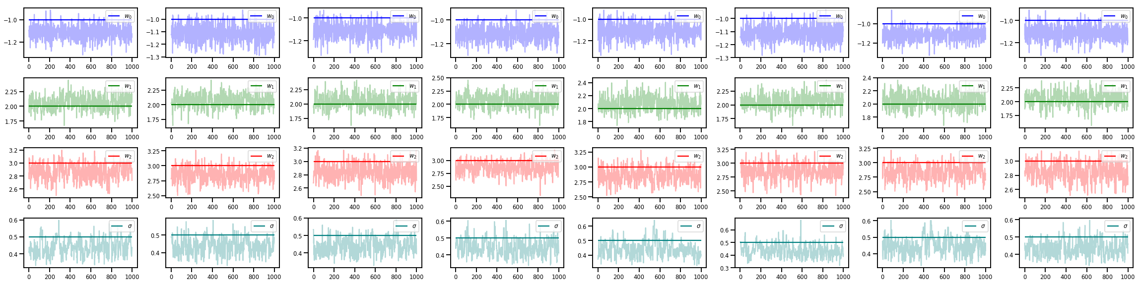
w_chains, sigma_chains = chains

# Trace plots of w (one of 8 chains)
colors = ['b', 'g', 'r', 'teal']
fig, axes = plt.subplots(4, num_chains, figsize=(4 * num_chains, 8))
for j in range(num_chains):
  for i in range(3):
    ax = axes[i][j]
    ax.plot(w_chains[:, j, i], c=colors[i], alpha=.3)
    ax.hlines(true_w[i], 0, 1000, zorder=4, color=colors[i], label="$w_{}$".format(i))
    ax.legend(loc='upper right')
  ax = axes[3][j]
  ax.plot(sigma_chains[:, j], alpha=.3, c=colors[3])
  ax.hlines(noise_scale, 0, 1000, zorder=4, color=colors[3], label=r"$\sigma$".format(i))
  ax.legend(loc='upper right')
fig.tight_layout()
plt.show()

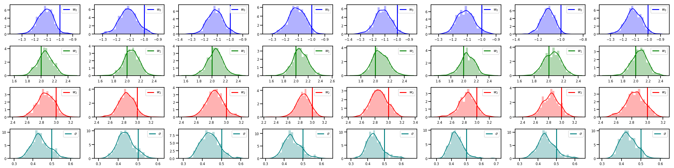
# Histogram of samples of w
fig, axes = plt.subplots(4, num_chains, figsize=(4 * num_chains, 8))
for j in range(num_chains):
  for i in range(3):
    ax = axes[i][j]
    sns.distplot(w_chains[:, j, i], color=colors[i], norm_hist=True, ax=ax, hist_kws={'alpha': .3})
  for i in range(3):
    ax = axes[i][j]
    ymax = ax.get_ylim()[1]
    ax.vlines(true_w[i], 0, ymax, color=colors[i], label="$w_{}$".format(i), linewidth=3)
    ax.set_ylim(0, ymax)
    ax.legend(loc='upper right')


  ax = axes[3][j]
  sns.distplot(sigma_chains[:, j], color=colors[3], norm_hist=True, ax=ax, hist_kws={'alpha': .3})
  ymax = ax.get_ylim()[1]
  ax.vlines(noise_scale, 0, ymax, color=colors[3], label=r"$\sigma$".format(i), linewidth=3)
  ax.set_ylim(0, ymax)
  ax.legend(loc='upper right')
fig.tight_layout()
plt.show()

มีอีกมาก!

ตรวจสอบโพสต์บล็อกและตัวอย่างที่ยอดเยี่ยมเหล่านี้:

• โครงสร้างอนุกรมเวลาการสนับสนุน บล็อก Colab
• ความน่าจะเป็น Keras เลเยอร์ (input: Tensor เอาท์พุท: การกระจาย!) บล็อก Colab
  • อีกตัวอย่างที่ชั้น: Vaes บล็อก Colab
• Gaussian กระบวนการถดถอย Colab และตัวแปรแฝงการสร้างแบบจำลอง Colab

ตัวอย่างเพิ่มเติมและโน๊ตบุ๊คบน GitHub ของเรา ที่นี่ !