
| | |  ดูแหล่งที่มาบน GitHub ดูแหล่งที่มาบน GitHub | |
ใน colab นี้ เราจะสำรวจการสุ่มตัวอย่างจากส่วนหลังของ Bayesian Gaussian Mixture Model (BGMM) โดยใช้เฉพาะค่าพื้นฐานความน่าจะเป็นของ TensorFlow เท่านั้น
แบบอย่าง
สำหรับ \(k\in\{1,\ldots, K\}\) ส่วนประกอบส่วนผสมแต่ละมิติ \(D\)เราต้องการรูปแบบ \(i\in\{1,\ldots,N\}\) IID ตัวอย่างใช้ต่อไปนี้คชกรรมเสียนผสมแบบ:
\[\begin{align*} \theta &\sim \text{Dirichlet}(\text{concentration}=\alpha_0)\\ \mu_k &\sim \text{Normal}(\text{loc}=\mu_{0k}, \text{scale}=I_D)\\ T_k &\sim \text{Wishart}(\text{df}=5, \text{scale}=I_D)\\ Z_i &\sim \text{Categorical}(\text{probs}=\theta)\\ Y_i &\sim \text{Normal}(\text{loc}=\mu_{z_i}, \text{scale}=T_{z_i}^{-1/2})\\ \end{align*}\]
หมายเหตุที่ scale ขัดแย้งทั้งหมดมี cholesky ความหมาย เราใช้แบบแผนนี้เพราะเป็นแบบแผนของ TF Distributions (ซึ่งตัวมันเองใช้แบบแผนนี้ในส่วนหนึ่งเพราะมันเป็นข้อได้เปรียบในการคำนวณ)
เป้าหมายของเราคือการสร้างตัวอย่างจากด้านหลัง:
\[p\left(\theta, \{\mu_k, T_k\}_{k=1}^K \Big| \{y_i\}_{i=1}^N, \alpha_0, \{\mu_{ok}\}_{k=1}^K\right)\]
ขอให้สังเกตว่า \(\{Z_i\}_{i=1}^N\) ไม่อยู่ - ได้เลยสนใจในเพียงตัวแปรสุ่มที่ไม่ขนาดกับ \(N\)(และโชคดีที่มีการกระจาย TF ซึ่งจัดการ marginalizing ออก \(Z_i\).)
เป็นไปไม่ได้ที่จะสุ่มตัวอย่างโดยตรงจากการแจกแจงนี้เนื่องจากเงื่อนไขการทำให้เป็นมาตรฐานที่คำนวณได้ยาก
อัลกอริทึมมหานครเฮสติ้งส์ เป็นเทคนิคสำหรับการสุ่มตัวอย่างจากการกระจายว่ายากต่อการปกติ
ความน่าจะเป็นของ TensorFlow มีตัวเลือก MCMC มากมาย รวมถึงตัวเลือกต่างๆ ตาม Metropolis-Hastings ในสมุดบันทึกนี้เราจะใช้ มิล Monte Carlo ( tfp.mcmc.HamiltonianMonteCarlo ) HMC มักเป็นทางเลือกที่ดีเพราะสามารถมาบรรจบกันได้อย่างรวดเร็ว สุ่มตัวอย่างพื้นที่ของรัฐร่วมกัน (ซึ่งต่างจากพิกัดเชิงพิกัด) และใช้ประโยชน์จากข้อดีประการหนึ่งของ TF: การแยกความแตกต่างโดยอัตโนมัติ ที่กล่าวว่าการสุ่มตัวอย่างจากหลัง BGMM จริงอาจทำได้ดีขึ้นโดยวิธีการอื่น ๆ เช่น กิบบ์ของการสุ่มตัวอย่าง
%matplotlib inline


import functools

import matplotlib.pyplot as plt; plt.style.use('ggplot')
import numpy as np
import seaborn as sns; sns.set_context('notebook')

import tensorflow.compat.v2 as tf
tf.enable_v2_behavior()
import tensorflow_probability as tfp

tfd = tfp.distributions
tfb = tfp.bijectors

physical_devices = tf.config.experimental.list_physical_devices('GPU')
if len(physical_devices) > 0:
  tf.config.experimental.set_memory_growth(physical_devices[0], True)
ก่อนสร้างแบบจำลองจริงๆ เราจะต้องกำหนดรูปแบบการแจกจ่ายใหม่ จากข้อกำหนดของแบบจำลองข้างต้น เห็นได้ชัดว่าเรากำลังกำหนดพารามิเตอร์ MVN ด้วยเมทริกซ์ความแปรปรวนร่วมผกผัน กล่าวคือ [เมทริกซ์ความแม่นยำ](https://en.wikipedia.org/wiki/Precision_(statistics%29) เพื่อให้บรรลุสิ่งนี้ใน TF เราจะต้องแผ่ออกของเรา Bijector นี้. Bijector จะใช้การเปลี่ยนแปลงไปข้างหน้า:
-
Y = tf.linalg.triangular_solve((tf.linalg.matrix_transpose(chol_precision_tril), X, adjoint=True) + loc
และ log_prob คำนวณเป็นเพียงสิ่งที่ตรงกันข้ามคือ:
-
X = tf.linalg.matmul(chol_precision_tril, X - loc, adjoint_a=True)
เนื่องจากทุกคนต้องเราสำหรับ HMC เป็น log_prob วิธีนี้เราหลีกเลี่ยงที่เคยเรียก tf.linalg.triangular_solve (เท่าที่จะเป็นกรณีสำหรับ tfd.MultivariateNormalTriL ) นี้เป็นข้อได้เปรียบตั้งแต่ tf.linalg.matmul มักจะได้เร็วขึ้นเนื่องจากท้องที่แคชที่ดีกว่า
class MVNCholPrecisionTriL(tfd.TransformedDistribution):
  """MVN from loc and (Cholesky) precision matrix."""

  def __init__(self, loc, chol_precision_tril, name=None):
    super(MVNCholPrecisionTriL, self).__init__(
        distribution=tfd.Independent(tfd.Normal(tf.zeros_like(loc),
                                                scale=tf.ones_like(loc)),
                                     reinterpreted_batch_ndims=1),
        bijector=tfb.Chain([
            tfb.Shift(shift=loc),
            tfb.Invert(tfb.ScaleMatvecTriL(scale_tril=chol_precision_tril,
                                           adjoint=True)),
        ]),
        name=name)
tfd.Independent ผลัดกระจายอิสระดึงของการกระจายหนึ่งลงไปในการกระจายหลายตัวแปรอิสระด้วยพิกัดทางสถิติ ในแง่ของการคำนวณ log_prob นี้ "เมตากระจาย" ปรากฏเป็นผลรวมที่เรียบง่ายมากกว่ามิติเหตุการณ์ (s)
นอกจากนี้ยังเห็นว่าเราเอา adjoint ( "transpose") ของเมทริกซ์ขนาด เพราะถ้ามีความแม่นยำเป็นแปรปรวนผกผันคือ \(P=C^{-1}\) และถ้า \(C=AA^\top\)แล้ว \(P=BB^{\top}\) ที่ \(B=A^{-\top}\)
ตั้งแต่การกระจายนี้เป็นชนิดของหากินให้ได้อย่างรวดเร็วตรวจสอบว่าเรา MVNCholPrecisionTriL ทำงานในขณะที่เราคิดว่ามันควรจะเป็น
def compute_sample_stats(d, seed=42, n=int(1e6)):
  x = d.sample(n, seed=seed)
  sample_mean = tf.reduce_mean(x, axis=0, keepdims=True)
  s = x - sample_mean
  sample_cov = tf.linalg.matmul(s, s, adjoint_a=True) / tf.cast(n, s.dtype)
  sample_scale = tf.linalg.cholesky(sample_cov)
  sample_mean = sample_mean[0]
  return [
      sample_mean,
      sample_cov,
      sample_scale,
  ]

dtype = np.float32
true_loc = np.array([1., -1.], dtype=dtype)
true_chol_precision = np.array([[1., 0.],
                                [2., 8.]],
                               dtype=dtype)
true_precision = np.matmul(true_chol_precision, true_chol_precision.T)
true_cov = np.linalg.inv(true_precision)

d = MVNCholPrecisionTriL(
    loc=true_loc,
    chol_precision_tril=true_chol_precision)

[sample_mean, sample_cov, sample_scale] = [
    t.numpy() for t in compute_sample_stats(d)]

print('true mean:', true_loc)
print('sample mean:', sample_mean)
print('true cov:\n', true_cov)
print('sample cov:\n', sample_cov)
true mean: [ 1. -1.]
sample mean: [ 1.0002806 -1.000105 ]
true cov:
 [[ 1.0625   -0.03125 ]
 [-0.03125   0.015625]]
sample cov:
 [[ 1.0641273  -0.03126175]
 [-0.03126175  0.01559312]]
เนื่องจากค่าเฉลี่ยตัวอย่างและความแปรปรวนร่วมนั้นใกล้เคียงกับค่าเฉลี่ยและความแปรปรวนร่วมที่แท้จริง ดูเหมือนว่าการกระจายจะถูกนำไปใช้อย่างถูกต้อง ตอนนี้เราจะใช้ MVNCholPrecisionTriL tfp.distributions.JointDistributionNamed เพื่อระบุรูปแบบ BGMM สำหรับรูปแบบการสังเกตเราจะใช้ tfd.MixtureSameFamily ที่จะบูรณาการโดยอัตโนมัติ \(\{Z_i\}_{i=1}^N\) ดึง
dtype = np.float64
dims = 2
components = 3
num_samples = 1000
bgmm = tfd.JointDistributionNamed(dict(
  mix_probs=tfd.Dirichlet(
    concentration=np.ones(components, dtype) / 10.),
  loc=tfd.Independent(
    tfd.Normal(
        loc=np.stack([
            -np.ones(dims, dtype),
            np.zeros(dims, dtype),
            np.ones(dims, dtype),
        ]),
        scale=tf.ones([components, dims], dtype)),
    reinterpreted_batch_ndims=2),
  precision=tfd.Independent(
    tfd.WishartTriL(
        df=5,
        scale_tril=np.stack([np.eye(dims, dtype=dtype)]*components),
        input_output_cholesky=True),
    reinterpreted_batch_ndims=1),
  s=lambda mix_probs, loc, precision: tfd.Sample(tfd.MixtureSameFamily(
      mixture_distribution=tfd.Categorical(probs=mix_probs),
      components_distribution=MVNCholPrecisionTriL(
          loc=loc,
          chol_precision_tril=precision)),
      sample_shape=num_samples)
))
def joint_log_prob(observations, mix_probs, loc, chol_precision):
  """BGMM with priors: loc=Normal, precision=Inverse-Wishart, mix=Dirichlet.

  Args:
    observations: `[n, d]`-shaped `Tensor` representing Bayesian Gaussian
      Mixture model draws. Each sample is a length-`d` vector.
    mix_probs: `[K]`-shaped `Tensor` representing random draw from
      `Dirichlet` prior.
    loc: `[K, d]`-shaped `Tensor` representing the location parameter of the
      `K` components.
    chol_precision: `[K, d, d]`-shaped `Tensor` representing `K` lower
      triangular `cholesky(Precision)` matrices, each being sampled from
      a Wishart distribution.

  Returns:
    log_prob: `Tensor` representing joint log-density over all inputs.
  """
  return bgmm.log_prob(
      mix_probs=mix_probs, loc=loc, precision=chol_precision, s=observations)
สร้างข้อมูล "การฝึกอบรม"
สำหรับการสาธิตนี้ เราจะสุ่มตัวอย่างข้อมูลบางส่วน
true_loc = np.array([[-2., -2],
                     [0, 0],
                     [2, 2]], dtype)
random = np.random.RandomState(seed=43)

true_hidden_component = random.randint(0, components, num_samples)
observations = (true_loc[true_hidden_component] +
                random.randn(num_samples, dims).astype(dtype))
การอนุมานแบบเบย์โดยใช้ HMC
ตอนนี้เราได้ใช้ TFD เพื่อระบุโมเดลของเราและได้รับข้อมูลที่สังเกตได้บางส่วนแล้ว เรามีส่วนที่จำเป็นทั้งหมดในการรัน HMC
การทำเช่นนี้เราจะใช้ แอพลิเคชันบางส่วน ที่ "ขาลง" สิ่งที่เราทำไม่ได้ต้องการตัวอย่าง ในกรณีนี้หมายความว่าเราจะต้องตอกตะปูลง observations (The-พารามิเตอร์มากเกินไปจะอบอยู่แล้วในการที่จะกระจายก่อนและไม่ได้เป็นส่วนหนึ่งของ joint_log_prob ลายเซ็นของฟังก์ชั่น.)
unnormalized_posterior_log_prob = functools.partial(joint_log_prob, observations)
initial_state = [
    tf.fill([components],
            value=np.array(1. / components, dtype),
            name='mix_probs'),
    tf.constant(np.array([[-2., -2],
                          [0, 0],
                          [2, 2]], dtype),
                name='loc'),
    tf.linalg.eye(dims, batch_shape=[components], dtype=dtype, name='chol_precision'),
]
การเป็นตัวแทนที่ไม่มีข้อจำกัด
Hamiltonian Monte Carlo (HMC) ต้องการฟังก์ชันความน่าจะเป็นบันทึกเป้าหมายที่สามารถหาอนุพันธ์ได้โดยใช้ข้อโต้แย้ง นอกจากนี้ HMC สามารถแสดงประสิทธิภาพทางสถิติที่สูงขึ้นอย่างมากหากพื้นที่ของรัฐไม่มีข้อจำกัด
ซึ่งหมายความว่าเราจะต้องแก้ไขปัญหาหลักสองประเด็นเมื่อสุ่มตัวอย่างจากส่วนหลังของ BGMM:
- \(\theta\) แสดงให้เห็นถึงความน่าจะเป็นเวกเตอร์โดยสิ้นเชิงกล่าวคือจะต้องเป็นเช่นนั้น \(\sum_{k=1}^K \theta_k = 1\) และ \(\theta_k>0\)
- \(T_k\) แสดงให้เห็นถึงความแปรปรวนเมทริกซ์ผกผันคือจะต้องเป็นเช่นนั้น \(T_k \succ 0\)คือเป็น บวกแน่นอน
เพื่อแก้ไขข้อกำหนดนี้ เราจะต้อง:
- เปลี่ยนตัวแปรที่ถูกจำกัดให้เป็นช่องว่างที่ไม่มีข้อจำกัด
- เรียกใช้ MCMC ในพื้นที่ที่ไม่มีข้อจำกัด
- เปลี่ยนตัวแปร unconstrained กลับไปเป็น contrained space
เช่นเดียวกับ MVNCholPrecisionTriL เราจะใช้ Bijector s จะเปลี่ยนตัวแปรสุ่มไปยังพื้นที่ไม่มีข้อ จำกัด
Dirichletจะเปลี่ยนไปยังพื้นที่ข้อ จำกัด ผ่าน ฟังก์ชั่น softmaxตัวแปรสุ่มที่มีความแม่นยำของเราคือการแจกแจงบนเมทริกซ์กึ่งกำหนดผลบวก หากต้องการยกเลิกการยึดเหล่านี้เราจะใช้
FillTriangularและTransformDiagonalbijectors สิ่งเหล่านี้แปลงเวกเตอร์เป็นเมทริกซ์สามเหลี่ยมล่างและให้แน่ใจว่าเส้นทแยงมุมเป็นค่าบวก อดีตจะเป็นประโยชน์เพราะจะช่วยให้การสุ่มตัวอย่างเพียง \(d(d+1)/2\) ลอยมากกว่า \(d^2\)
unconstraining_bijectors = [
    tfb.SoftmaxCentered(),
    tfb.Identity(),
    tfb.Chain([
        tfb.TransformDiagonal(tfb.Softplus()),
        tfb.FillTriangular(),
    ])]
@tf.function(autograph=False)
def sample():
  return tfp.mcmc.sample_chain(
    num_results=2000,
    num_burnin_steps=500,
    current_state=initial_state,
    kernel=tfp.mcmc.SimpleStepSizeAdaptation(
        tfp.mcmc.TransformedTransitionKernel(
            inner_kernel=tfp.mcmc.HamiltonianMonteCarlo(
                target_log_prob_fn=unnormalized_posterior_log_prob,
                 step_size=0.065,
                 num_leapfrog_steps=5),
            bijector=unconstraining_bijectors),
         num_adaptation_steps=400),
    trace_fn=lambda _, pkr: pkr.inner_results.inner_results.is_accepted)

[mix_probs, loc, chol_precision], is_accepted = sample()
ตอนนี้เราจะดำเนินการห่วงโซ่และพิมพ์วิธีการด้านหลัง
acceptance_rate = tf.reduce_mean(tf.cast(is_accepted, dtype=tf.float32)).numpy()
mean_mix_probs = tf.reduce_mean(mix_probs, axis=0).numpy()
mean_loc = tf.reduce_mean(loc, axis=0).numpy()
mean_chol_precision = tf.reduce_mean(chol_precision, axis=0).numpy()
precision = tf.linalg.matmul(chol_precision, chol_precision, transpose_b=True)
print('acceptance_rate:', acceptance_rate)
print('avg mix probs:', mean_mix_probs)
print('avg loc:\n', mean_loc)
print('avg chol(precision):\n', mean_chol_precision)
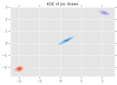
acceptance_rate: 0.5305
avg mix probs: [0.25248723 0.60729516 0.1402176 ]
avg loc:
 [[-1.96466753 -2.12047249]
 [ 0.27628865  0.22944732]
 [ 2.06461244  2.54216122]]
avg chol(precision):
 [[[ 1.05105032  0.        ]
  [ 0.12699955  1.06553113]]

 [[ 0.76058015  0.        ]
  [-0.50332767  0.77947431]]

 [[ 1.22770457  0.        ]
  [ 0.70670027  1.50914164]]]
loc_ = loc.numpy()
ax = sns.kdeplot(loc_[:,0,0], loc_[:,0,1], shade=True, shade_lowest=False)
ax = sns.kdeplot(loc_[:,1,0], loc_[:,1,1], shade=True, shade_lowest=False)
ax = sns.kdeplot(loc_[:,2,0], loc_[:,2,1], shade=True, shade_lowest=False)
plt.title('KDE of loc draws');
บทสรุป
colab แบบง่ายๆ นี้แสดงให้เห็นวิธีที่ TensorFlow Probability primitives สามารถใช้เพื่อสร้างแบบจำลองส่วนผสม Bayesian แบบมีลำดับชั้น