| | |  ดูแหล่งที่มาบน GitHub ดูแหล่งที่มาบน GitHub | |
โน๊ตบุ๊คนี้ reimplements และขยาย“การวิเคราะห์จุดเปลี่ยน” คชกรรมตัวอย่างจาก เอกสาร pymc3
ข้อกำหนดเบื้องต้น
import tensorflow.compat.v2 as tf
tf.enable_v2_behavior()
import tensorflow_probability as tfp
tfd = tfp.distributions
tfb = tfp.bijectors
import matplotlib.pyplot as plt
plt.rcParams['figure.figsize'] = (15,8)
%config InlineBackend.figure_format = 'retina'
import numpy as np
import pandas as pd
ชุดข้อมูล
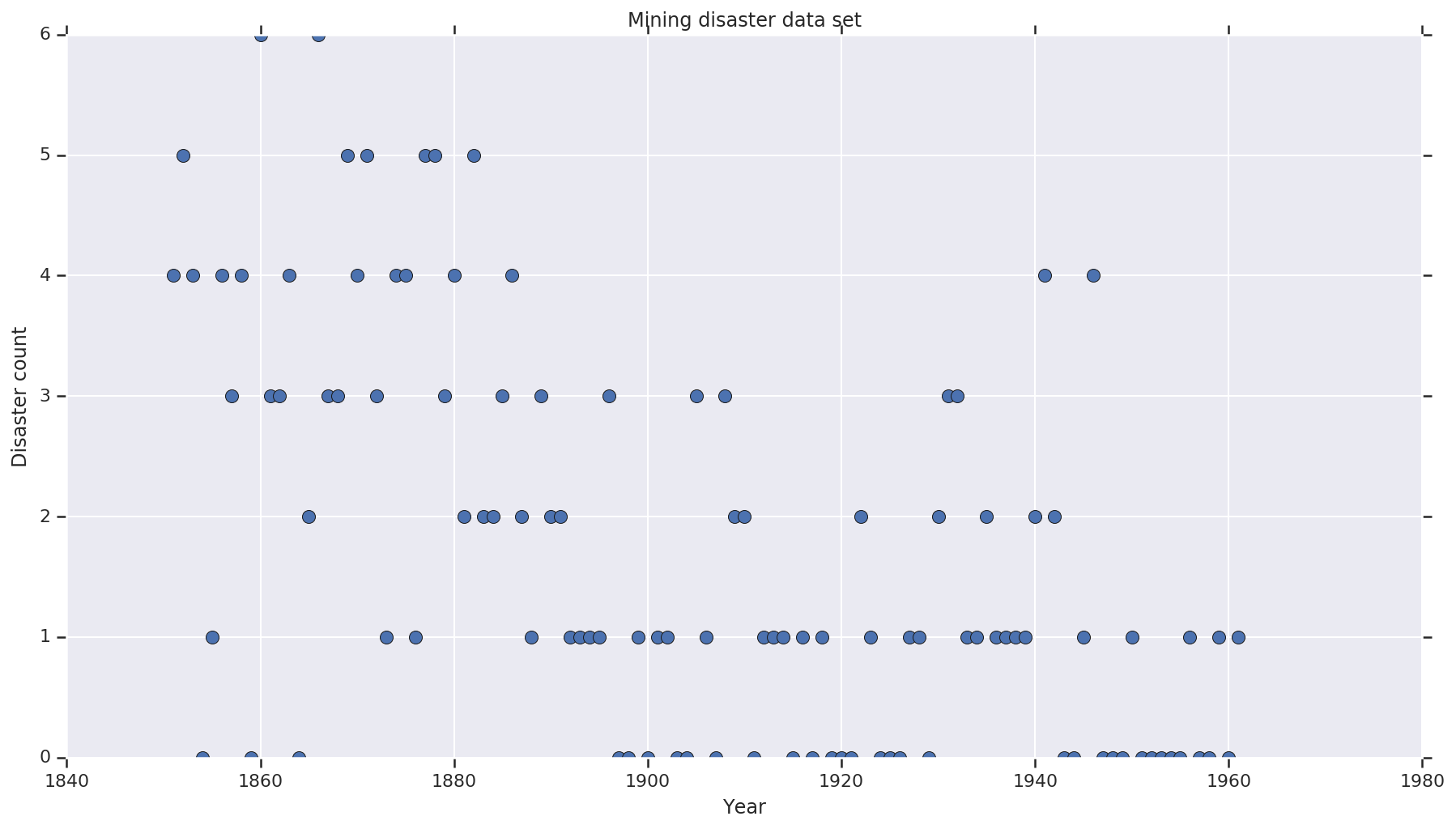
ชุดข้อมูลจาก ที่นี่ หมายเหตุมีรุ่นของตัวอย่างนี้อีก ลอยรอบ แต่มันก็มี“หายไป” ข้อมูล - ซึ่งในกรณีนี้คุณจะต้องใส่ร้ายค่าที่ขาดหายไป (มิฉะนั้น โมเดลของคุณจะไม่มีวันทิ้งพารามิเตอร์เริ่มต้นไว้ เนื่องจากฟังก์ชันความน่าจะเป็นจะไม่ได้กำหนดไว้)
disaster_data = np.array([ 4, 5, 4, 0, 1, 4, 3, 4, 0, 6, 3, 3, 4, 0, 2, 6,
                           3, 3, 5, 4, 5, 3, 1, 4, 4, 1, 5, 5, 3, 4, 2, 5,
                           2, 2, 3, 4, 2, 1, 3, 2, 2, 1, 1, 1, 1, 3, 0, 0,
                           1, 0, 1, 1, 0, 0, 3, 1, 0, 3, 2, 2, 0, 1, 1, 1,
                           0, 1, 0, 1, 0, 0, 0, 2, 1, 0, 0, 0, 1, 1, 0, 2,
                           3, 3, 1, 1, 2, 1, 1, 1, 1, 2, 4, 2, 0, 0, 1, 4,
                           0, 0, 0, 1, 0, 0, 0, 0, 0, 1, 0, 0, 1, 0, 1])
years = np.arange(1851, 1962)
plt.plot(years, disaster_data, 'o', markersize=8);
plt.ylabel('Disaster count')
plt.xlabel('Year')
plt.title('Mining disaster data set')
plt.show()
แบบจำลองความน่าจะเป็น
แบบจำลองนี้ถือว่า "จุดเปลี่ยน" (เช่น ปีที่มีการเปลี่ยนแปลงกฎข้อบังคับด้านความปลอดภัย) และอัตราภัยพิบัติที่กระจายปัวซองด้วยอัตราคงที่ (แต่อาจแตกต่างออกไป) ก่อนและหลังจุดเปลี่ยนนั้น
จำนวนภัยพิบัติที่แท้จริงได้รับการแก้ไข (สังเกต) ตัวอย่างของโมเดลนี้จะต้องระบุทั้งจุดสวิตช์และอัตราการเกิดภัยพิบัติ "ต้น" และ "ปลาย"
รูปแบบเดิมจาก ตัวอย่างเอกสาร pymc3 :
\[ \begin{align*} (D_t|s,e,l)&\sim \text{Poisson}(r_t), \\ & \,\quad\text{with}\; r_t = \begin{cases}e & \text{if}\; t < s\\l &\text{if}\; t \ge s\end{cases} \\ s&\sim\text{Discrete Uniform}(t_l,\,t_h) \\ e&\sim\text{Exponential}(r_e)\\ l&\sim\text{Exponential}(r_l) \end{align*} \]
อย่างไรก็ตามค่าเฉลี่ยอัตราการเกิดภัยพิบัติ \(r_t\) มีต่อเนื่องที่ switchpoint \(s\)ซึ่งจะทำให้มันไม่อนุพันธ์ ดังนั้นมันจึงไม่ได้ให้สัญญาณการไล่ระดับสีเพื่ออัลกอริทึม (HMC) มิล Monte Carlo - แต่เพราะ \(s\) ก่อนเป็นอย่างต่อเนื่องทางเลือกของ HMC จะสุ่มเดินก็เพียงพอที่ดีที่จะหาพื้นที่ของมวลความน่าจะเป็นสูงในตัวอย่างนี้
ในฐานะที่เป็นรุ่นที่สองเราปรับเปลี่ยนรูปแบบเดิมโดยใช้ sigmoid“สวิทช์” ระหว่าง E และ L ที่จะทำให้การเปลี่ยนแปลงอนุพันธ์และใช้เครื่องแบบกระจายอย่างต่อเนื่องสำหรับ switchpoint \(s\)(อาจมีคนโต้แย้งว่าแบบจำลองนี้เป็นจริงมากกว่าความเป็นจริง เนื่องจาก "สวิตช์" ในอัตราเฉลี่ยน่าจะยืดเยื้อไปหลายปี) โมเดลใหม่นี้มีลักษณะดังนี้:
\[ \begin{align*} (D_t|s,e,l)&\sim\text{Poisson}(r_t), \\ & \,\quad \text{with}\; r_t = e + \frac{1}{1+\exp(s-t)}(l-e) \\ s&\sim\text{Uniform}(t_l,\,t_h) \\ e&\sim\text{Exponential}(r_e)\\ l&\sim\text{Exponential}(r_l) \end{align*} \]
ในกรณีที่ไม่มีข้อมูลเพิ่มเติมที่เราถือว่า \(r_e = r_l = 1\) เป็นพารามิเตอร์สำหรับไพรเออร์ เราจะเรียกใช้ทั้งสองโมเดลและเปรียบเทียบผลการอนุมาน
def disaster_count_model(disaster_rate_fn):
  disaster_count = tfd.JointDistributionNamed(dict(
    e=tfd.Exponential(rate=1.),
    l=tfd.Exponential(rate=1.),
    s=tfd.Uniform(0., high=len(years)),
    d_t=lambda s, l, e: tfd.Independent(
        tfd.Poisson(rate=disaster_rate_fn(np.arange(len(years)), s, l, e)),
        reinterpreted_batch_ndims=1)
  ))
  return disaster_count

def disaster_rate_switch(ys, s, l, e):
  return tf.where(ys < s, e, l)

def disaster_rate_sigmoid(ys, s, l, e):
  return e + tf.sigmoid(ys - s) * (l - e)

model_switch = disaster_count_model(disaster_rate_switch)
model_sigmoid = disaster_count_model(disaster_rate_sigmoid)
โค้ดด้านบนกำหนดโมเดลผ่านการแจกแจง JointDistributionSequential disaster_rate ฟังก์ชั่นที่เรียกว่ากับอาร์เรย์ของ [0, ..., len(years)-1] การผลิตเวกเตอร์ของ len(years) ตัวแปรสุ่ม - ปีก่อนที่ switchpoint มี early_disaster_rate คนหลังจาก late_disaster_rate (โมดูโล การเปลี่ยนซิกมอยด์)
นี่คือการตรวจสอบสติว่าฟังก์ชันบันทึกเป้าหมายมีเหตุผล:
def target_log_prob_fn(model, s, e, l):
  return model.log_prob(s=s, e=e, l=l, d_t=disaster_data)

models = [model_switch, model_sigmoid]
print([target_log_prob_fn(m, 40., 3., .9).numpy() for m in models])  # Somewhat likely result
print([target_log_prob_fn(m, 60., 1., 5.).numpy() for m in models])  # Rather unlikely result
print([target_log_prob_fn(m, -10., 1., 1.).numpy() for m in models]) # Impossible result
[-176.94559, -176.28717]
[-371.3125, -366.8816]
[-inf, -inf]
HMC ทำการอนุมานแบบเบย์
เรากำหนดจำนวนผลลัพธ์และขั้นตอนเบิร์นอินที่จำเป็น รหัสเป็นแบบจำลองส่วนใหญ่หลังจากที่ เอกสารของ tfp.mcmc.HamiltonianMonteCarlo มันใช้ขนาดขั้นตอนที่ปรับได้ (มิฉะนั้นผลลัพธ์จะอ่อนไหวมากกับค่าขนาดขั้นตอนที่เลือก) เราใช้ค่าหนึ่งเป็นสถานะเริ่มต้นของลูกโซ่
นี่ไม่ใช่เรื่องราวทั้งหมดแม้ว่า หากคุณกลับไปที่คำจำกัดความของแบบจำลองด้านบน คุณจะสังเกตว่าการแจกแจงความน่าจะเป็นบางตัวไม่ได้กำหนดไว้อย่างดีบนเส้นจำนวนจริงทั้งหมด ดังนั้นเราจึง จำกัด พื้นที่ที่ HMC จะต้องตรวจสอบโดยการตัดเคอร์เนล HMC ด้วย TransformedTransitionKernel ที่ระบุ bijectors ไปข้างหน้าเพื่อเปลี่ยนตัวเลขจริงบนโดเมนที่กระจายความน่าจะถูกกำหนดไว้ใน (ดูความคิดเห็นในรหัสด้านล่าง)
num_results = 10000
num_burnin_steps = 3000

@tf.function(autograph=False, jit_compile=True)
def make_chain(target_log_prob_fn):
   kernel = tfp.mcmc.TransformedTransitionKernel(
       inner_kernel=tfp.mcmc.HamiltonianMonteCarlo(
          target_log_prob_fn=target_log_prob_fn,
          step_size=0.05,
          num_leapfrog_steps=3),
       bijector=[
          # The switchpoint is constrained between zero and len(years).
          # Hence we supply a bijector that maps the real numbers (in a
          # differentiable way) to the interval (0;len(yers))
          tfb.Sigmoid(low=0., high=tf.cast(len(years), dtype=tf.float32)),
          # Early and late disaster rate: The exponential distribution is
          # defined on the positive real numbers
          tfb.Softplus(),
          tfb.Softplus(),
      ])
   kernel = tfp.mcmc.SimpleStepSizeAdaptation(
        inner_kernel=kernel,
        num_adaptation_steps=int(0.8*num_burnin_steps))

   states = tfp.mcmc.sample_chain(
      num_results=num_results,
      num_burnin_steps=num_burnin_steps,
      current_state=[
          # The three latent variables
          tf.ones([], name='init_switchpoint'),
          tf.ones([], name='init_early_disaster_rate'),
          tf.ones([], name='init_late_disaster_rate'),
      ],
      trace_fn=None,
      kernel=kernel)
   return states

switch_samples = [s.numpy() for s in make_chain(
    lambda *args: target_log_prob_fn(model_switch, *args))]
sigmoid_samples = [s.numpy() for s in make_chain(
    lambda *args: target_log_prob_fn(model_sigmoid, *args))]

switchpoint, early_disaster_rate, late_disaster_rate = zip(
    switch_samples, sigmoid_samples)
เรียกใช้ทั้งสองรุ่นพร้อมกัน:
เห็นภาพผลลัพธ์
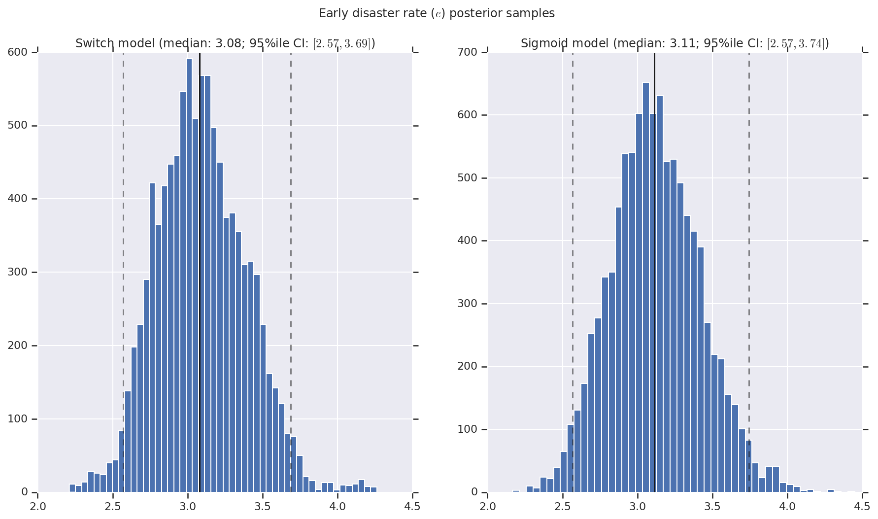
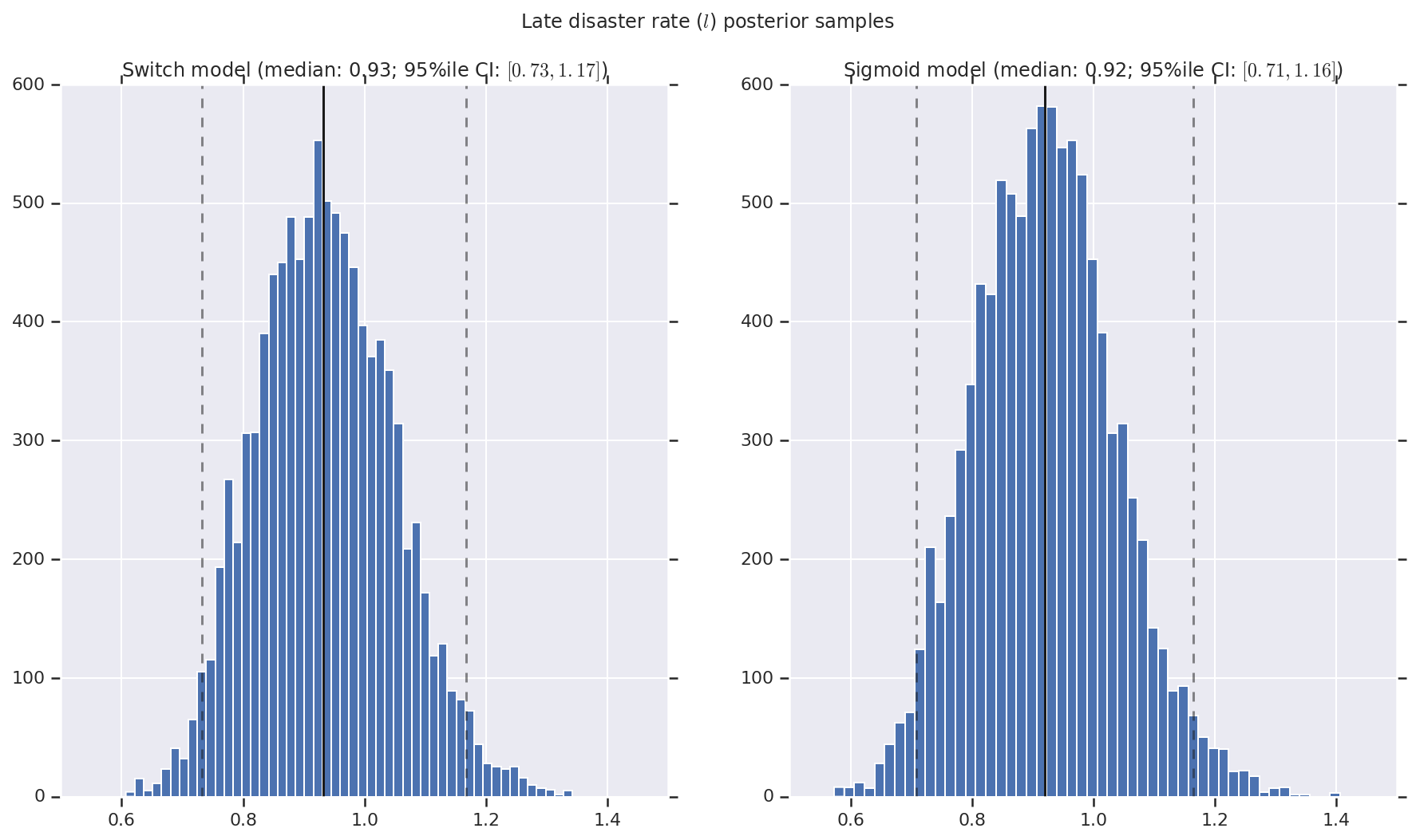
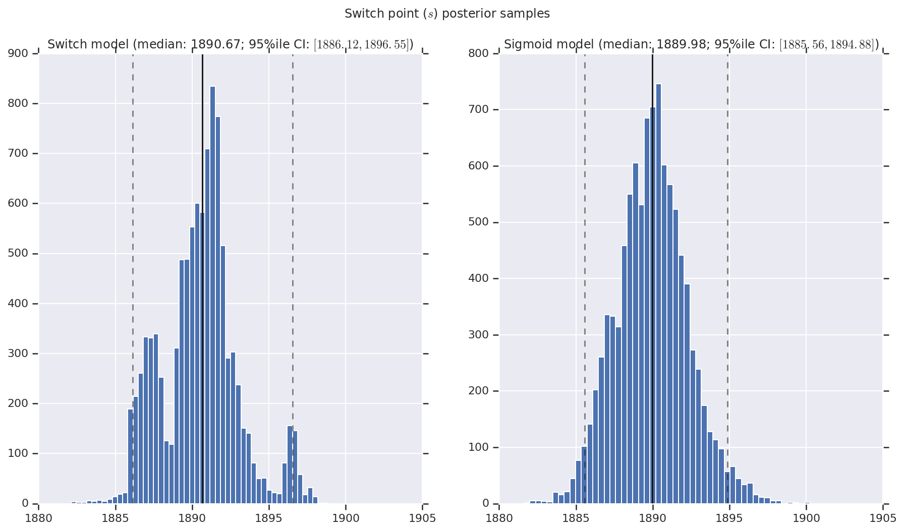
เราเห็นภาพผลลัพธ์เป็นฮิสโตแกรมของตัวอย่างของการกระจายภายหลังสำหรับอัตราการเกิดภัยพิบัติช่วงต้นและปลาย ตลอดจนจุดเปลี่ยน ฮิสโตแกรมถูกซ้อนทับด้วยเส้นทึบที่แสดงถึงค่ามัธยฐานของตัวอย่าง เช่นเดียวกับขอบเขตช่วงที่น่าเชื่อถือ 95% เป็นเส้นประ
def _desc(v):
  return '(median: {}; 95%ile CI: $[{}, {}]$)'.format(
      *np.round(np.percentile(v, [50, 2.5, 97.5]), 2))

for t, v in [
    ('Early disaster rate ($e$) posterior samples', early_disaster_rate),
    ('Late disaster rate ($l$) posterior samples', late_disaster_rate),
    ('Switch point ($s$) posterior samples', years[0] + switchpoint),
]:
  fig, ax = plt.subplots(nrows=1, ncols=2, sharex=True)
  for (m, i) in (('Switch', 0), ('Sigmoid', 1)):
    a = ax[i]
    a.hist(v[i], bins=50)
    a.axvline(x=np.percentile(v[i], 50), color='k')
    a.axvline(x=np.percentile(v[i], 2.5), color='k', ls='dashed', alpha=.5)
    a.axvline(x=np.percentile(v[i], 97.5), color='k', ls='dashed', alpha=.5)
    a.set_title(m + ' model ' + _desc(v[i]))
  fig.suptitle(t)
  plt.show()