
| | |  ดูแหล่งที่มาบน GitHub ดูแหล่งที่มาบน GitHub | |
ติดตั้ง
ขั้นแรกให้ติดตั้งแพ็คเกจที่ใช้ในการสาธิตนี้
pip install -q dm-sonnet
การนำเข้า (tf, tfp พร้อมเคล็ดลับที่อยู่ติดกัน ฯลฯ )
import numpy as np
import tqdm as tqdm
import sklearn.datasets as skd

# visualization
import matplotlib.pyplot as plt
import seaborn as sns
from scipy.stats import kde

# tf and friends
import tensorflow.compat.v2 as tf
import tensorflow_probability as tfp
import sonnet as snt
tf.enable_v2_behavior()

tfb = tfp.bijectors
tfd = tfp.distributions

def make_grid(xmin, xmax, ymin, ymax, gridlines, pts):
  xpts = np.linspace(xmin, xmax, pts)
  ypts = np.linspace(ymin, ymax, pts)
  xgrid = np.linspace(xmin, xmax, gridlines)
  ygrid = np.linspace(ymin, ymax, gridlines)
  xlines = np.stack([a.ravel() for a in np.meshgrid(xpts, ygrid)])
  ylines = np.stack([a.ravel() for a in np.meshgrid(xgrid, ypts)])
  return np.concatenate([xlines, ylines], 1).T

grid = make_grid(-3, 3, -3, 3, 4, 100)
/usr/local/lib/python3.6/dist-packages/statsmodels/tools/_testing.py:19: FutureWarning: pandas.util.testing is deprecated. Use the functions in the public API at pandas.testing instead.
  import pandas.util.testing as tm
ฟังก์ชันตัวช่วยสำหรับการแสดงภาพ
def plot_density(data, axis):
  x, y = np.squeeze(np.split(data, 2, axis=1))
  levels = np.linspace(0.0, 0.75, 10)
  kwargs = {'levels': levels}
  return sns.kdeplot(x, y, cmap="viridis", shade=True,
                     shade_lowest=True, ax=axis, **kwargs)


def plot_points(data, axis, s=10, color='b', label=''):
  x, y = np.squeeze(np.split(data, 2, axis=1))
  axis.scatter(x, y, c=color, s=s, label=label)


def plot_panel(
    grid, samples, transformed_grid, transformed_samples,
    dataset, axarray, limits=True):
  if len(axarray) != 4:
    raise ValueError('Expected 4 axes for the panel')
  ax1, ax2, ax3, ax4 = axarray
  plot_points(data=grid, axis=ax1, s=20, color='black', label='grid')
  plot_points(samples, ax1, s=30, color='blue', label='samples')
  plot_points(transformed_grid, ax2, s=20, color='black', label='ode(grid)')
  plot_points(transformed_samples, ax2, s=30, color='blue', label='ode(samples)')
  ax3 = plot_density(transformed_samples, ax3)
  ax4 = plot_density(dataset, ax4)
  if limits:
    set_limits([ax1], -3.0, 3.0, -3.0, 3.0)
    set_limits([ax2], -2.0, 3.0, -2.0, 3.0)
    set_limits([ax3, ax4], -1.5, 2.5, -0.75, 1.25)


def set_limits(axes, min_x, max_x, min_y, max_y):
  if isinstance(axes, list):
    for axis in axes:
      set_limits(axis, min_x, max_x, min_y, max_y)
  else:
    axes.set_xlim(min_x, max_x)
    axes.set_ylim(min_y, max_y)
FFJORD bijector
ใน colab นี้ เราสาธิต FFJORD bijector ซึ่งเสนอครั้งแรกในบทความโดย Grathwohl, Will, et al การเชื่อมโยง arXiv
สรุปความคิดที่อยู่เบื้องหลังวิธีการดังกล่าวคือการสร้างการติดต่อระหว่างการกระจายฐานที่รู้จักกันและการกระจายข้อมูล
ในการสร้างการเชื่อมต่อนี้ เราต้อง
- กำหนดแผนที่ bijective \(\mathcal{T}_{\theta}:\mathbf{x} \rightarrow \mathbf{y}\), \(\mathcal{T}_{\theta}^{1}:\mathbf{y} \rightarrow \mathbf{x}\) ระหว่างพื้นที่ \(\mathcal{Y}\) ที่กระจายฐานถูกกำหนดและพื้นที่ \(\mathcal{X}\) โดเมนข้อมูล
- ได้อย่างมีประสิทธิภาพในการติดตามของรูปร่างที่เราดำเนินการถ่ายโอนความคิดของความน่าจะเป็นบน \(\mathcal{X}\)
เงื่อนไขที่สองจะอยู่ในกรงเล็บนิพจน์ต่อไปนี้สำหรับการกระจายความน่าจะกำหนดไว้ใน \(\mathcal{X}\):
\[ \log p_{\mathbf{x} }(\mathbf{x})=\log p_{\mathbf{y} }(\mathbf{y})-\log \operatorname{det}\left|\frac{\partial \mathcal{T}_{\theta}(\mathbf{y})}{\partial \mathbf{y} }\right| \]
FFJORD bijector บรรลุสิ่งนี้โดยการกำหนดการแปลง
\[ \mathcal{T_{\theta} }: \mathbf{x} = \mathbf{z}(t_{0}) \rightarrow \mathbf{y} = \mathbf{z}(t_{1}) \quad : \quad \frac{d \mathbf{z} }{dt} = \mathbf{f}(t, \mathbf{z}, \theta) \]
การเปลี่ยนแปลงครั้งนี้เป็นผกผันได้ตราบใดที่ฟังก์ชั่น \(\mathbf{f}\) อธิบายวิวัฒนาการของรัฐ \(\mathbf{z}\) จะประพฤติดีและ log_det_jacobian สามารถคำนวณได้โดยการบูรณาการการแสดงออกดังต่อไปนี้
\[ \log \operatorname{det}\left|\frac{\partial \mathcal{T}_{\theta}(\mathbf{y})}{\partial \mathbf{y} }\right| = -\int_{t_{0} }^{t_{1} } \operatorname{Tr}\left(\frac{\partial \mathbf{f}(t, \mathbf{z}, \theta)}{\partial \mathbf{z}(t)}\right) d t \]
ในการสาธิตนี้เราจะมาฝึกอบรม bijector FFJORD การวาร์ปการกระจายเกาส์เข้าสู่การจัดจำหน่ายที่กำหนดโดย moons ชุด สิ่งนี้จะทำใน 3 ขั้นตอน:
- กําหนดการกระจายฐาน
- กำหนด FFJORD bijector
- ลดโอกาสบันทึกที่แน่นอนของชุดข้อมูล
ขั้นแรก เราโหลด data
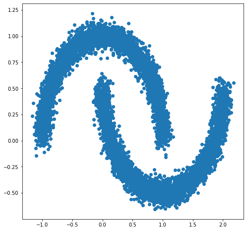
ชุดข้อมูล
DATASET_SIZE = 1024 * 8
BATCH_SIZE = 256
SAMPLE_SIZE = DATASET_SIZE

moons = skd.make_moons(n_samples=DATASET_SIZE, noise=.06)[0]

moons_ds = tf.data.Dataset.from_tensor_slices(moons.astype(np.float32))
moons_ds = moons_ds.prefetch(tf.data.experimental.AUTOTUNE)
moons_ds = moons_ds.cache()
moons_ds = moons_ds.shuffle(DATASET_SIZE)
moons_ds = moons_ds.batch(BATCH_SIZE)

plt.figure(figsize=[8, 8])
plt.scatter(moons[:, 0], moons[:, 1])
plt.show()
ต่อไป เรายกตัวอย่างการกระจายฐาน
base_loc = np.array([0.0, 0.0]).astype(np.float32)
base_sigma = np.array([0.8, 0.8]).astype(np.float32)
base_distribution = tfd.MultivariateNormalDiag(base_loc, base_sigma)
เราใช้หลายชั้นตรอนกับรูปแบบ state_derivative_fn
ในขณะที่ไม่จำเป็นสำหรับชุดนี้ก็มักจะ benefitial เพื่อให้ state_derivative_fn ขึ้นอยู่กับเวลา ที่นี่เราบรรลุนี้โดยเชื่อมโยง t ปัจจัยการผลิตของเครือข่ายของเรา
class MLP_ODE(snt.Module):
  """Multi-layer NN ode_fn."""
  def __init__(self, num_hidden, num_layers, num_output, name='mlp_ode'):
    super(MLP_ODE, self).__init__(name=name)
    self._num_hidden = num_hidden
    self._num_output = num_output
    self._num_layers = num_layers
    self._modules = []
    for _ in range(self._num_layers - 1):
      self._modules.append(snt.Linear(self._num_hidden))
      self._modules.append(tf.math.tanh)
    self._modules.append(snt.Linear(self._num_output))
    self._model = snt.Sequential(self._modules)

  def __call__(self, t, inputs):
    inputs = tf.concat([tf.broadcast_to(t, inputs.shape), inputs], -1)
    return self._model(inputs)
พารามิเตอร์แบบจำลองและการฝึกอบรม
LR = 1e-2
NUM_EPOCHS = 80
STACKED_FFJORDS = 4
NUM_HIDDEN = 8
NUM_LAYERS = 3
NUM_OUTPUT = 2
ตอนนี้เราสร้างสแต็กของ FFJORD bijectors แต่ละ bijector มีให้กับ ode_solve_fn และ trace_augmentation_fn และเป็นของตัวเอง state_derivative_fn รุ่นเพื่อที่พวกเขาจะแสดงลำดับของการเปลี่ยนแปลงที่แตกต่างกัน
ตัวสร้างไบเจ็คเตอร์
solver = tfp.math.ode.DormandPrince(atol=1e-5)
ode_solve_fn = solver.solve
trace_augmentation_fn = tfb.ffjord.trace_jacobian_exact

bijectors = []
for _ in range(STACKED_FFJORDS):
  mlp_model = MLP_ODE(NUM_HIDDEN, NUM_LAYERS, NUM_OUTPUT)
  next_ffjord = tfb.FFJORD(
      state_time_derivative_fn=mlp_model,ode_solve_fn=ode_solve_fn,
      trace_augmentation_fn=trace_augmentation_fn)
  bijectors.append(next_ffjord)

stacked_ffjord = tfb.Chain(bijectors[::-1])
ตอนนี้เราสามารถใช้ TransformedDistribution ซึ่งเป็นผลมาจากการแปรปรวน base_distribution กับ stacked_ffjord bijector
transformed_distribution = tfd.TransformedDistribution(
    distribution=base_distribution, bijector=stacked_ffjord)
ตอนนี้เรากำหนดขั้นตอนการฝึกอบรมของเรา เราเพียงแค่ลดโอกาสในการบันทึกเชิงลบของข้อมูล
การฝึกอบรม
@tf.function
def train_step(optimizer, target_sample):
  with tf.GradientTape() as tape:
    loss = -tf.reduce_mean(transformed_distribution.log_prob(target_sample))
  variables = tape.watched_variables()
  gradients = tape.gradient(loss, variables)
  optimizer.apply(gradients, variables)
  return loss
ตัวอย่าง
@tf.function
def get_samples():
  base_distribution_samples = base_distribution.sample(SAMPLE_SIZE)
  transformed_samples = transformed_distribution.sample(SAMPLE_SIZE)
  return base_distribution_samples, transformed_samples


@tf.function
def get_transformed_grid():
  transformed_grid = stacked_ffjord.forward(grid)
  return transformed_grid
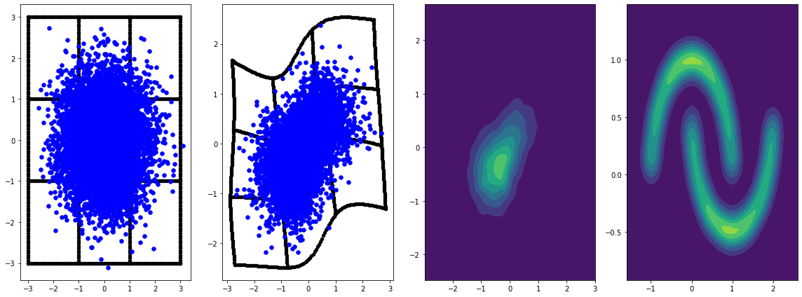
พล็อตตัวอย่างจากฐานและการกระจายที่แปลงแล้ว
evaluation_samples = []
base_samples, transformed_samples = get_samples()
transformed_grid = get_transformed_grid()
evaluation_samples.append((base_samples, transformed_samples, transformed_grid))
WARNING:tensorflow:From /usr/local/lib/python3.6/dist-packages/tensorflow/python/ops/resource_variable_ops.py:1817: calling BaseResourceVariable.__init__ (from tensorflow.python.ops.resource_variable_ops) with constraint is deprecated and will be removed in a future version.
Instructions for updating:
If using Keras pass *_constraint arguments to layers.
panel_id = 0
panel_data = evaluation_samples[panel_id]
fig, axarray = plt.subplots(
  1, 4, figsize=(16, 6))
plot_panel(
    grid, panel_data[0], panel_data[2], panel_data[1], moons, axarray, False)
plt.tight_layout()
learning_rate = tf.Variable(LR, trainable=False)
optimizer = snt.optimizers.Adam(learning_rate)

for epoch in tqdm.trange(NUM_EPOCHS // 2):
  base_samples, transformed_samples = get_samples()
  transformed_grid = get_transformed_grid()
  evaluation_samples.append(
      (base_samples, transformed_samples, transformed_grid))
  for batch in moons_ds:
    _ = train_step(optimizer, batch)
0%|          | 0/40 [00:00<?, ?it/s]
WARNING:tensorflow:From /usr/local/lib/python3.6/dist-packages/tensorflow_probability/python/math/ode/base.py:350: calling while_loop_v2 (from tensorflow.python.ops.control_flow_ops) with back_prop=False is deprecated and will be removed in a future version.
Instructions for updating:
back_prop=False is deprecated. Consider using tf.stop_gradient instead.
Instead of:
results = tf.while_loop(c, b, vars, back_prop=False)
Use:
results = tf.nest.map_structure(tf.stop_gradient, tf.while_loop(c, b, vars))
100%|██████████| 40/40 [07:00<00:00, 10.52s/it]
panel_id = -1
panel_data = evaluation_samples[panel_id]
fig, axarray = plt.subplots(
  1, 4, figsize=(16, 6))
plot_panel(grid, panel_data[0], panel_data[2], panel_data[1], moons, axarray)
plt.tight_layout()
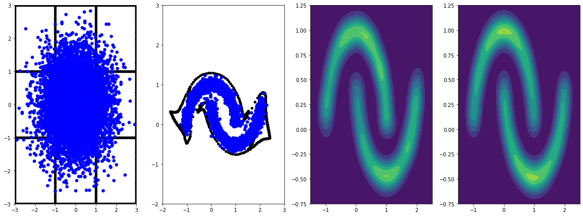
การฝึกอบรมให้นานขึ้นด้วยอัตราการเรียนรู้ส่งผลให้มีการปรับปรุงเพิ่มเติม
ไม่ได้แปลงในตัวอย่างนี้ FFJORD bijector รองรับการประมาณค่า stochastic trace ของ hutchinson ประมาณการโดยเฉพาะอย่างยิ่งสามารถให้บริการผ่านทาง trace_augmentation_fn ในทำนองเดียวกันติดทางเลือกที่สามารถนำมาใช้โดยการกำหนดที่กำหนดเอง ode_solve_fn