
| | |  ดูแหล่งที่มาบน GitHub ดูแหล่งที่มาบน GitHub | |
ติดตั้ง
TF_Installation = 'System'

if TF_Installation == 'TF Nightly':
  !pip install -q --upgrade tf-nightly
  print('Installation of `tf-nightly` complete.')
elif TF_Installation == 'TF Stable':
  !pip install -q --upgrade tensorflow
  print('Installation of `tensorflow` complete.')
elif TF_Installation == 'System':
  pass
else:
  raise ValueError('Selection Error: Please select a valid '
                   'installation option.')
ติดตั้ง
TFP_Installation = "System"

if TFP_Installation == "Nightly":
  !pip install -q tfp-nightly
  print("Installation of `tfp-nightly` complete.")
elif TFP_Installation == "Stable":
  !pip install -q --upgrade tensorflow-probability
  print("Installation of `tensorflow-probability` complete.")
elif TFP_Installation == "System":
  pass
else:
  raise ValueError("Selection Error: Please select a valid "
                   "installation option.")
เชิงนามธรรม
ใน colab นี้ เราสาธิตวิธีปรับโมเดลเอฟเฟกต์ผสมเชิงเส้นทั่วไปโดยใช้การอนุมานความแปรปรวนในความน่าจะเป็นของ TensorFlow
โมเดลครอบครัว
ทั่วไปเชิงเส้นรุ่นผสมผล (GLMM) มีความคล้ายคลึงกับ ทั่วไปเส้นตรงรุ่น (GLM) ยกเว้นว่าพวกเขารวมเสียงตัวอย่างที่เฉพาะเจาะจงลงไปในการตอบสนองเชิงเส้นที่คาดการณ์ไว้ สิ่งนี้มีประโยชน์ส่วนหนึ่งเพราะทำให้ฟีเจอร์ที่ไม่ค่อยได้เห็นสามารถแชร์ข้อมูลกับฟีเจอร์ที่เห็นได้ทั่วไป
ในฐานะที่เป็นกระบวนการกำเนิด แบบจำลองเอฟเฟกต์ผสมเชิงเส้นทั่วไป (GLMM) มีลักษณะเฉพาะโดย:
\[ \begin{align} \text{for } & r = 1\ldots R: \hspace{2.45cm}\text{# for each random-effect group}\\ &\begin{aligned} \text{for } &c = 1\ldots |C_r|: \hspace{1.3cm}\text{# for each category ("level") of group $r$}\\ &\begin{aligned} \beta_{rc} &\sim \text{MultivariateNormal}(\text{loc}=0_{D_r}, \text{scale}=\Sigma_r^{1/2}) \end{aligned} \end{aligned}\\\\ \text{for } & i = 1 \ldots N: \hspace{2.45cm}\text{# for each sample}\\ &\begin{aligned} &\eta_i = \underbrace{\vphantom{\sum_{r=1}^R}x_i^\top\omega}_\text{fixed-effects} + \underbrace{\sum_{r=1}^R z_{r,i}^\top \beta_{r,C_r(i) } }_\text{random-effects} \\ &Y_i|x_i,\omega,\{z_{r,i} , \beta_r\}_{r=1}^R \sim \text{Distribution}(\text{mean}= g^{-1}(\eta_i)) \end{aligned} \end{align} \]
ที่ไหน:
\[ \begin{align} R &= \text{number of random-effect groups}\\ |C_r| &= \text{number of categories for group $r$}\\ N &= \text{number of training samples}\\ x_i,\omega &\in \mathbb{R}^{D_0}\\ D_0 &= \text{number of fixed-effects}\\ C_r(i) &= \text{category (under group $r$) of the $i$th sample}\\ z_{r,i} &\in \mathbb{R}^{D_r}\\ D_r &= \text{number of random-effects associated with group $r$}\\ \Sigma_{r} &\in \{S\in\mathbb{R}^{D_r \times D_r} : S \succ 0 \}\\ \eta_i\mapsto g^{-1}(\eta_i) &= \mu_i, \text{inverse link function}\\ \text{Distribution} &=\text{some distribution parameterizable solely by its mean} \end{align} \]
ในคำอื่น ๆ นี้บอกว่าหมวดหมู่ของแต่ละกลุ่มทุกคนจะเกี่ยวข้องกับตัวอย่าง \(\beta_{rc}\)จากหลายตัวแปรปกติ แม้ว่า \(\beta_{rc}\) ดึงอยู่เสมออิสระพวกเขาเป็นเพียงการกระจาย indentically สำหรับกลุ่ม \(r\): แจ้งให้ทราบล่วงหน้ามีตรงหนึ่ง \(\Sigma_r\) สำหรับแต่ละ \(r\in\{1,\ldots,R\}\)
เมื่อรวม affinely ที่มีคุณสมบัติของกลุ่มตัวอย่างของ (\(z_{r,i}\)) ผลที่ได้คือเสียงตัวอย่างเฉพาะใน \(i\)-th คาดการณ์การตอบสนองเชิงเส้น (ซึ่งเป็นตัวเลขที่มิฉะนั้น \(x_i^\top\omega\))
เมื่อเราประเมิน \(\{\Sigma_r:r\in\{1,\ldots,R\}\}\) เรากำลังหลักประเมินปริมาณของเสียงกลุ่มสุ่มผลดำเนินการซึ่งจะกลบในปัจจุบันสัญญาณใน \(x_i^\top\omega\)
มีความหลากหลายของตัวเลือกสำหรับการเป็น \(\text{Distribution}\) และ ฟังก์ชั่นการเชื่อมโยงผกผัน , \(g^{-1}\)ทางเลือกทั่วไปคือ:
- \(Y_i\sim\text{Normal}(\text{mean}=\eta_i, \text{scale}=\sigma)\),
- \(Y_i\sim\text{Binomial}(\text{mean}=n_i \cdot \text{sigmoid}(\eta_i), \text{total_count}=n_i)\)และ
- \(Y_i\sim\text{Poisson}(\text{mean}=\exp(\eta_i))\)
สำหรับความเป็นไปได้มากขึ้นดู tfp.glm โมดูล
การอนุมานแบบแปรผัน
แต่น่าเสียดายที่การหาค่าประมาณความน่าจะเป็นสูงสุดของพารามิเตอร์ \(\beta,\{\Sigma_r\}_r^R\) สร้างความสำคัญไม่ใช่การวิเคราะห์ เพื่อหลีกเลี่ยงปัญหานี้ เราแทน
- กำหนดครอบครัวแปรของการกระจาย (ที่ "ความหนาแน่นของตัวแทน") แสดง \(q_{\lambda}\) ในภาคผนวก
- ค้นหาพารามิเตอร์ \(\lambda\) เพื่อให้ \(q_{\lambda}\) อยู่ใกล้กับ denstiy เป้าหมายของเราจริง
ครอบครัวของการกระจายจะ Gaussians อิสระจากขนาดที่เหมาะสมและโดย "ใกล้กับความหนาแน่นของเป้าหมายของเรา" เราจะหมายถึง "การลด ความแตกต่าง Kullback-Leibler " ดูตัวอย่างเช่น มาตรา 2.2 ของ "แปรผันอนุมาน: Review สำหรับสถิติ" หามาเขียนดีและแรงจูงใจ โดยเฉพาะอย่างยิ่ง มันแสดงให้เห็นว่าการลดความแตกต่างของ KL ให้น้อยที่สุดนั้นเทียบเท่ากับการลดขอบเขตล่างของหลักฐานเชิงลบ (ELBO)
ปัญหาของเล่น
Gelman et al. ของ (2007) "ชุดเรดอน" เป็นชุดข้อมูลที่บางครั้งใช้ในการแสดงให้เห็นถึงวิธีการสำหรับการถดถอย (เช่นที่เกี่ยวข้องอย่างใกล้ชิดนี้ โพสต์บล็อก PyMC3 .) ชุดข้อมูลเรดอนมีการตรวจวัดน้ำในร่มของเรดอนนำทั่วประเทศสหรัฐอเมริกา เรดอน เป็นธรรมชาติ ocurring ก๊าซกัมมันตรังสีซึ่งเป็น พิษ ในระดับความเข้มข้นสูง
สำหรับการสาธิตของเรา สมมติว่าเราสนใจที่จะตรวจสอบสมมติฐานที่ว่าระดับเรดอนสูงกว่าในครัวเรือนที่มีห้องใต้ดิน นอกจากนี้เรายังสงสัยว่าความเข้มข้นของเรดอนเกี่ยวข้องกับชนิดของดิน กล่าวคือ เรื่องภูมิศาสตร์
ในการจัดกรอบนี้เป็นปัญหา ML เราจะพยายามคาดการณ์ระดับล็อก-เรดอนโดยพิจารณาจากฟังก์ชันเชิงเส้นของพื้นที่ใช้อ่านค่า นอกจากนี้ เราจะใช้เคาน์ตีเป็นเอฟเฟกต์แบบสุ่ม และด้วยเหตุนี้จึงพิจารณาความแปรปรวนอันเนื่องมาจากภูมิศาสตร์ ในคำอื่น ๆ เราจะใช้ ทั่วไปเชิงเส้นรูปแบบผสมผล
%matplotlib inline
%config InlineBackend.figure_format = 'retina'

import os
from six.moves import urllib

import matplotlib.pyplot as plt; plt.style.use('ggplot')
import numpy as np
import pandas as pd
import seaborn as sns; sns.set_context('notebook')
import tensorflow_datasets as tfds

import tensorflow.compat.v2 as tf
tf.enable_v2_behavior()

import tensorflow_probability as tfp
tfd = tfp.distributions
tfb = tfp.bijectors
เราจะทำการตรวจสอบความพร้อมใช้งานของ GPU อย่างรวดเร็ว:
if tf.test.gpu_device_name() != '/device:GPU:0':
  print("We'll just use the CPU for this run.")
else:
  print('Huzzah! Found GPU: {}'.format(tf.test.gpu_device_name()))
We'll just use the CPU for this run.
รับชุดข้อมูล:
เราโหลดชุดข้อมูลจากชุดข้อมูล TensorFlow และทำการประมวลผลล่วงหน้าเล็กน้อย
def load_and_preprocess_radon_dataset(state='MN'):
  """Load the Radon dataset from TensorFlow Datasets and preprocess it.

  Following the examples in "Bayesian Data Analysis" (Gelman, 2007), we filter
  to Minnesota data and preprocess to obtain the following features:
  - `county`: Name of county in which the measurement was taken.
  - `floor`: Floor of house (0 for basement, 1 for first floor) on which the
    measurement was taken.

  The target variable is `log_radon`, the log of the Radon measurement in the
  house.
  """
  ds = tfds.load('radon', split='train')
  radon_data = tfds.as_dataframe(ds)
  radon_data.rename(lambda s: s[9:] if s.startswith('feat') else s, axis=1, inplace=True)
  df = radon_data[radon_data.state==state.encode()].copy()

  df['radon'] = df.activity.apply(lambda x: x if x > 0. else 0.1)
  # Make county names look nice.
  df['county'] = df.county.apply(lambda s: s.decode()).str.strip().str.title()
  # Remap categories to start from 0 and end at max(category).
  df['county'] = df.county.astype(pd.api.types.CategoricalDtype())
  df['county_code'] = df.county.cat.codes
  # Radon levels are all positive, but log levels are unconstrained
  df['log_radon'] = df['radon'].apply(np.log)

  # Drop columns we won't use and tidy the index
  columns_to_keep = ['log_radon', 'floor', 'county', 'county_code']
  df = df[columns_to_keep].reset_index(drop=True)

  return df

df = load_and_preprocess_radon_dataset()
df.head()
เชี่ยวชาญในตระกูล GLMM
ในส่วนนี้ เราเชี่ยวชาญในตระกูล GLMM ในการทำนายระดับเรดอน ในการทำเช่นนี้ ก่อนอื่นเราพิจารณากรณีพิเศษที่มีเอฟเฟกต์คงที่ของ GLMM:
\[ \mathbb{E}[\log(\text{radon}_j)] = c + \text{floor_effect}_j \]
รุ่นนี้ posits ว่าเรดอนในบันทึกการสังเกต \(j\) คือ (ในความคาดหวัง) ควบคุมโดยพื้น \(j\)อ่าน TH มีการดำเนินการในการบวกบางสกัดกั้นอย่างต่อเนื่อง ใน pseudocode เราอาจเขียน
def estimate_log_radon(floor):
    return intercept + floor_effect[floor]
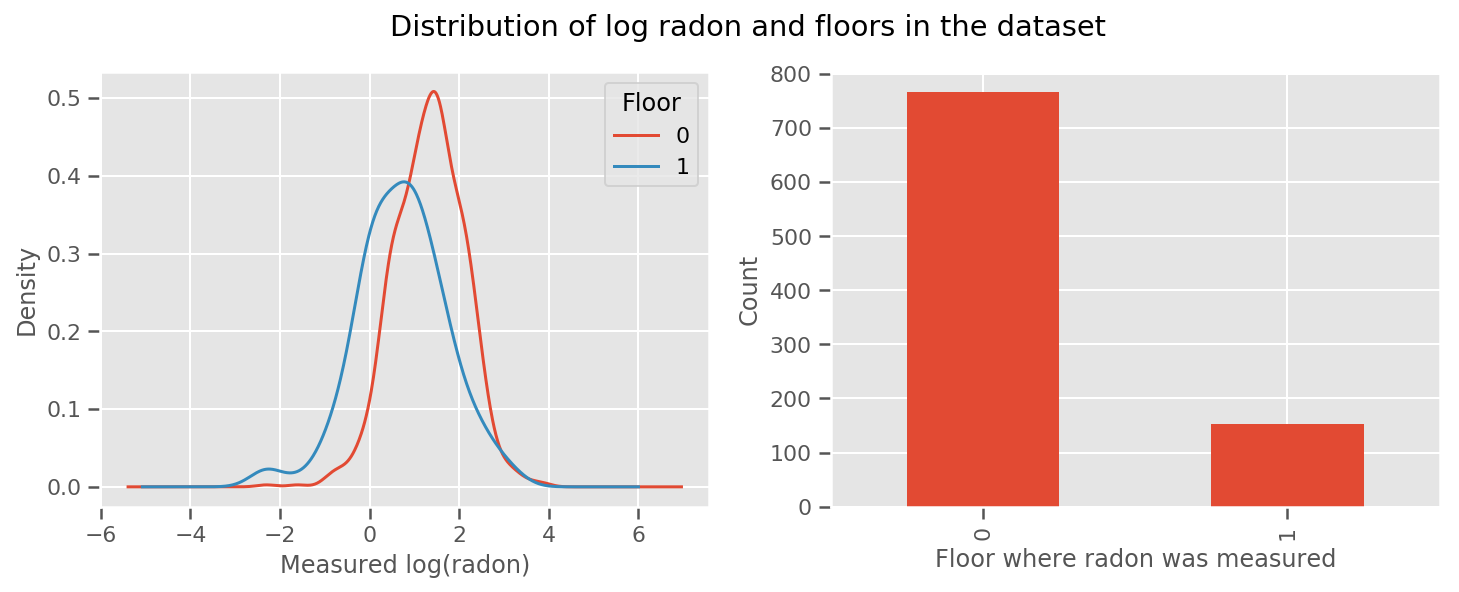
มีน้ำหนักเรียนรู้สำหรับทุกชั้นและสากล intercept ระยะ เมื่อดูการวัดเรดอนจากชั้น 0 และ 1 ดูเหมือนว่านี่อาจเป็นจุดเริ่มต้นที่ดี:
fig, (ax1, ax2) = plt.subplots(ncols=2, figsize=(12, 4))
df.groupby('floor')['log_radon'].plot(kind='density', ax=ax1);
ax1.set_xlabel('Measured log(radon)')
ax1.legend(title='Floor')

df['floor'].value_counts().plot(kind='bar', ax=ax2)
ax2.set_xlabel('Floor where radon was measured')
ax2.set_ylabel('Count')
fig.suptitle("Distribution of log radon and floors in the dataset");
ในการทำให้แบบจำลองซับซ้อนขึ้นเล็กน้อย ซึ่งรวมถึงบางอย่างเกี่ยวกับภูมิศาสตร์อาจจะดียิ่งขึ้นไปอีก: เรดอนเป็นส่วนหนึ่งของห่วงโซ่การสลายตัวของยูเรเนียม ซึ่งอาจมีอยู่บนพื้น ดังนั้นภูมิศาสตร์จึงดูเหมือนเป็นปัจจัยสำคัญ
\[ \mathbb{E}[\log(\text{radon}_j)] = c + \text{floor_effect}_j + \text{county_effect}_j \]
อีกครั้งใน pseudocode เรามี
def estimate_log_radon(floor, county):
    return intercept + floor_effect[floor] + county_effect[county]
เหมือนเดิม ยกเว้นน้ำหนักเฉพาะเขต
ด้วยชุดฝึกอบรมที่มีขนาดใหญ่พอสมควร นี่เป็นแบบจำลองที่สมเหตุสมผล อย่างไรก็ตาม จากข้อมูลของเราจากมินนิโซตา เราพบว่ามีเคาน์ตีจำนวนมากที่มีหน่วยวัดเพียงเล็กน้อย ตัวอย่างเช่น 39 จาก 85 มณฑลมีข้อสังเกตน้อยกว่าห้าแห่ง
สิ่งนี้กระตุ้นให้เกิดการแบ่งปันความแข็งแกร่งทางสถิติระหว่างการสังเกตทั้งหมดของเรา ในลักษณะที่บรรจบกับแบบจำลองข้างต้นเมื่อจำนวนการสังเกตต่อเขตเพิ่มขึ้น
fig, ax = plt.subplots(figsize=(22, 5));
county_freq = df['county'].value_counts()
county_freq.plot(kind='bar', ax=ax)
ax.set_xlabel('County')
ax.set_ylabel('Number of readings');
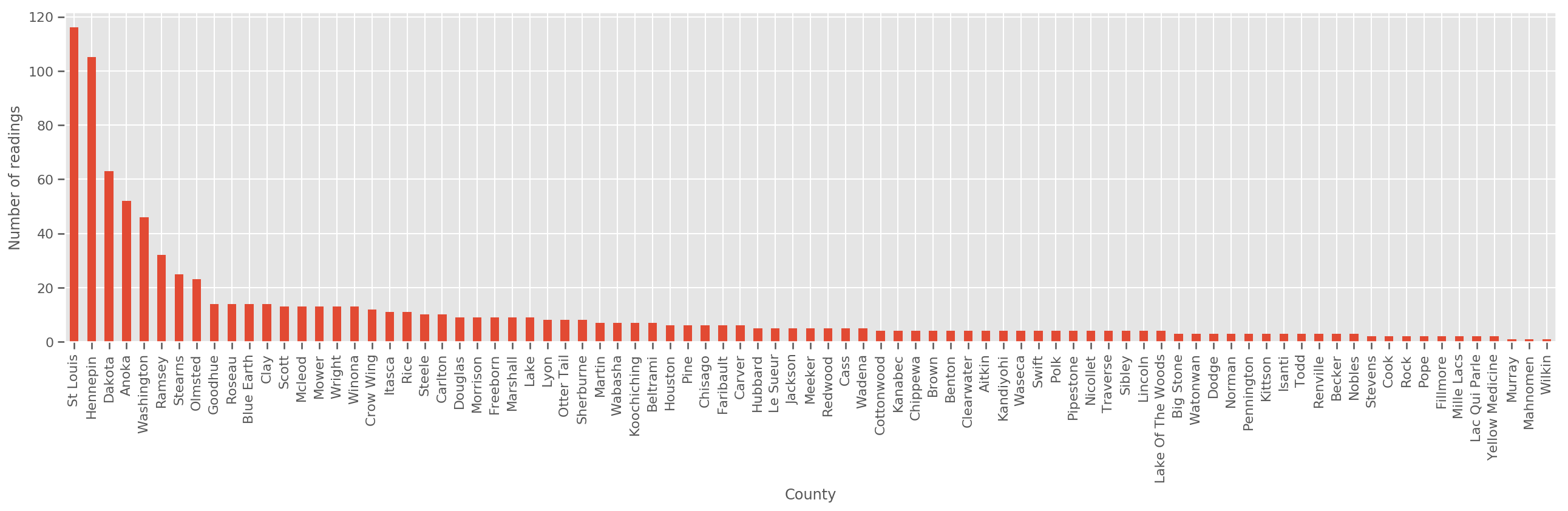
ถ้าเราเหมาะสมกับรูปแบบนี้ county_effect เวกเตอร์แนวโน้มที่จะจบลงด้วยการท่องจำผลสำหรับการปกครองซึ่งมีตัวอย่างการฝึกอบรมเพียงไม่กี่บางที overfitting และนำไปสู่การทั่วไปที่ไม่ดี
GLMM มอบความสุขระหว่างสอง GLM ข้างต้น เราอาจจะพิจารณาความเหมาะสม
\[ \log(\text{radon}_j) \sim c + \text{floor_effect}_j + \mathcal{N}(\text{county_effect}_j, \text{county_scale}) \]
รุ่นนี้เป็นเช่นเดียวกับครั้งแรก แต่เราได้รับการแก้ไขโอกาสของเราที่จะกระจายปกติและจะแบ่งปันความแปรปรวนทั่วทุกจังหวัดผ่าน (เดี่ยว) ตัวแปร county_scale ในรหัสเทียม
def estimate_log_radon(floor, county):
    county_mean = county_effect[county]
    random_effect = np.random.normal() * county_scale + county_mean
    return intercept + floor_effect[floor] + random_effect
เราจะสรุปร่วมกันจำหน่ายมากกว่า county_scale , county_mean และ random_effect โดยใช้ข้อมูลที่สังเกตของเรา ทั่วโลก county_scale ช่วยให้เราสามารถแบ่งปันความแข็งแรงทางสถิติทั่วมณฑล: ผู้ที่มีหลายข้อสังเกตให้ตีที่แปรปรวนของมณฑลที่มีไม่กี่ข้อสังเกตที่ นอกจากนี้ เมื่อเรารวบรวมข้อมูลมากขึ้น โมเดลนี้จะมาบรรจบกับโมเดลโดยไม่มีตัวแปรสเกลแบบรวม - แม้จะมีชุดข้อมูลนี้ เราก็จะได้ข้อสรุปที่คล้ายคลึงกันเกี่ยวกับเคาน์ตีที่สังเกตได้มากที่สุดด้วยโมเดลใดโมเดลหนึ่ง
การทดลอง
ตอนนี้เราจะพยายามปรับให้พอดีกับ GLMM ด้านบนโดยใช้การอนุมานแบบแปรผันใน TensorFlow อันดับแรก เราจะแบ่งข้อมูลออกเป็นคุณสมบัติและป้ายกำกับ
features = df[['county_code', 'floor']].astype(int)
labels = df[['log_radon']].astype(np.float32).values.flatten()
ระบุรุ่น
def make_joint_distribution_coroutine(floor, county, n_counties, n_floors):

  def model():
    county_scale = yield tfd.HalfNormal(scale=1., name='scale_prior')
    intercept = yield tfd.Normal(loc=0., scale=1., name='intercept')
    floor_weight = yield tfd.Normal(loc=0., scale=1., name='floor_weight')
    county_prior = yield tfd.Normal(loc=tf.zeros(n_counties),
                                    scale=county_scale,
                                    name='county_prior')
    random_effect = tf.gather(county_prior, county, axis=-1)

    fixed_effect = intercept + floor_weight * floor
    linear_response = fixed_effect + random_effect
    yield tfd.Normal(loc=linear_response, scale=1., name='likelihood')
  return tfd.JointDistributionCoroutineAutoBatched(model)

joint = make_joint_distribution_coroutine(
    features.floor.values, features.county_code.values, df.county.nunique(),
    df.floor.nunique())

# Define a closure over the joint distribution
# to condition on the observed labels.
def target_log_prob_fn(*args):
  return joint.log_prob(*args, likelihood=labels)
ระบุตัวแทนหลัง
ตอนนี้เราใส่กันในครอบครัวตัวแทน \(q_{\lambda}\)ที่พารามิเตอร์ \(\lambda\) มีสุวินัย ในกรณีนี้ครอบครัวของเรามีความเป็นอิสระกระจายหลายตัวแปรปกติหนึ่งสำหรับแต่ละพารามิเตอร์และ \(\lambda = \{(\mu_j, \sigma_j)\}\)ที่ \(j\) ดัชนีพารามิเตอร์ที่สี่
วิธีการที่เราใช้เพื่อให้เหมาะสมกับการใช้ตัวแทนครอบครัว tf.Variables เรายังใช้ tfp.util.TransformedVariable พร้อมกับ Softplus การ จำกัด (ที่สุวินัย) พารามิเตอร์ขนาดจะเป็นบวก นอกจากนี้เรายังใช้ Softplus ไปทั่ว scale_prior ซึ่งเป็นพารามิเตอร์ในเชิงบวก
เราเริ่มต้นตัวแปรที่ฝึกได้เหล่านี้ด้วยความกระวนกระวายใจเล็กน้อยเพื่อช่วยในการปรับให้เหมาะสม
# Initialize locations and scales randomly with `tf.Variable`s and
# `tfp.util.TransformedVariable`s.
_init_loc = lambda shape=(): tf.Variable(
    tf.random.uniform(shape, minval=-2., maxval=2.))
_init_scale = lambda shape=(): tfp.util.TransformedVariable(
    initial_value=tf.random.uniform(shape, minval=0.01, maxval=1.),
    bijector=tfb.Softplus())
n_counties = df.county.nunique()

surrogate_posterior = tfd.JointDistributionSequentialAutoBatched([
  tfb.Softplus()(tfd.Normal(_init_loc(), _init_scale())),           # scale_prior
  tfd.Normal(_init_loc(), _init_scale()),                           # intercept
  tfd.Normal(_init_loc(), _init_scale()),                           # floor_weight
  tfd.Normal(_init_loc([n_counties]), _init_scale([n_counties]))])  # county_prior
โปรดทราบว่ามือถือนี้สามารถถูกแทนที่ด้วย tfp.experimental.vi.build_factored_surrogate_posterior เช่น:
surrogate_posterior = tfp.experimental.vi.build_factored_surrogate_posterior(
  event_shape=joint.event_shape_tensor()[:-1],
  constraining_bijectors=[tfb.Softplus(), None, None, None])
ผล
จำไว้ว่าเป้าหมายของเราคือการกำหนดกลุ่มการแจกแจงแบบกำหนดพารามิเตอร์ที่ติดตามได้ จากนั้นเลือกพารามิเตอร์เพื่อให้เรามีการแจกแจงที่ติดตามได้ซึ่งใกล้เคียงกับการแจกแจงเป้าหมายของเรา
เราได้สร้างการกระจายตัวแทนข้างต้นและสามารถใช้ tfp.vi.fit_surrogate_posterior ซึ่งยอมรับเพิ่มประสิทธิภาพและจำนวนที่กำหนดของขั้นตอนในการหาพารามิเตอร์สำหรับรูปแบบตัวแทนที่ลด ELBO เชิงลบ (ซึ่ง corresonds เพื่อลดความแตกต่าง Kullback-Liebler ระหว่าง ตัวแทนและการกระจายเป้าหมาย)
ค่าตอบแทนเป็น ELBO เชิงลบในแต่ละขั้นตอนและการกระจายใน surrogate_posterior จะได้รับการปรับปรุงด้วยพารามิเตอร์ที่พบได้โดยการเพิ่มประสิทธิภาพ
optimizer = tf.optimizers.Adam(learning_rate=1e-2)

losses = tfp.vi.fit_surrogate_posterior(
    target_log_prob_fn,
    surrogate_posterior,
    optimizer=optimizer,
    num_steps=3000,
    seed=42,
    sample_size=2)

(scale_prior_,
 intercept_,
 floor_weight_,
 county_weights_), _ = surrogate_posterior.sample_distributions()
print('        intercept (mean): ', intercept_.mean())
print('     floor_weight (mean): ', floor_weight_.mean())
print(' scale_prior (approx. mean): ', tf.reduce_mean(scale_prior_.sample(10000)))
intercept (mean):  tf.Tensor(1.4352839, shape=(), dtype=float32)
     floor_weight (mean):  tf.Tensor(-0.6701997, shape=(), dtype=float32)
 scale_prior (approx. mean):  tf.Tensor(0.28682157, shape=(), dtype=float32)
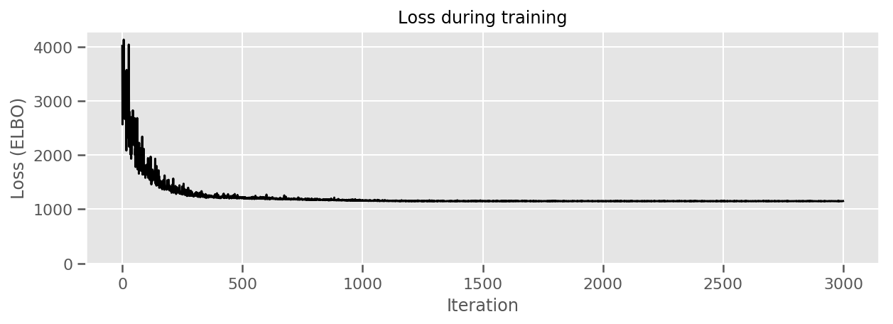
fig, ax = plt.subplots(figsize=(10, 3))
ax.plot(losses, 'k-')
ax.set(xlabel="Iteration",
       ylabel="Loss (ELBO)",
       title="Loss during training",
       ylim=0);
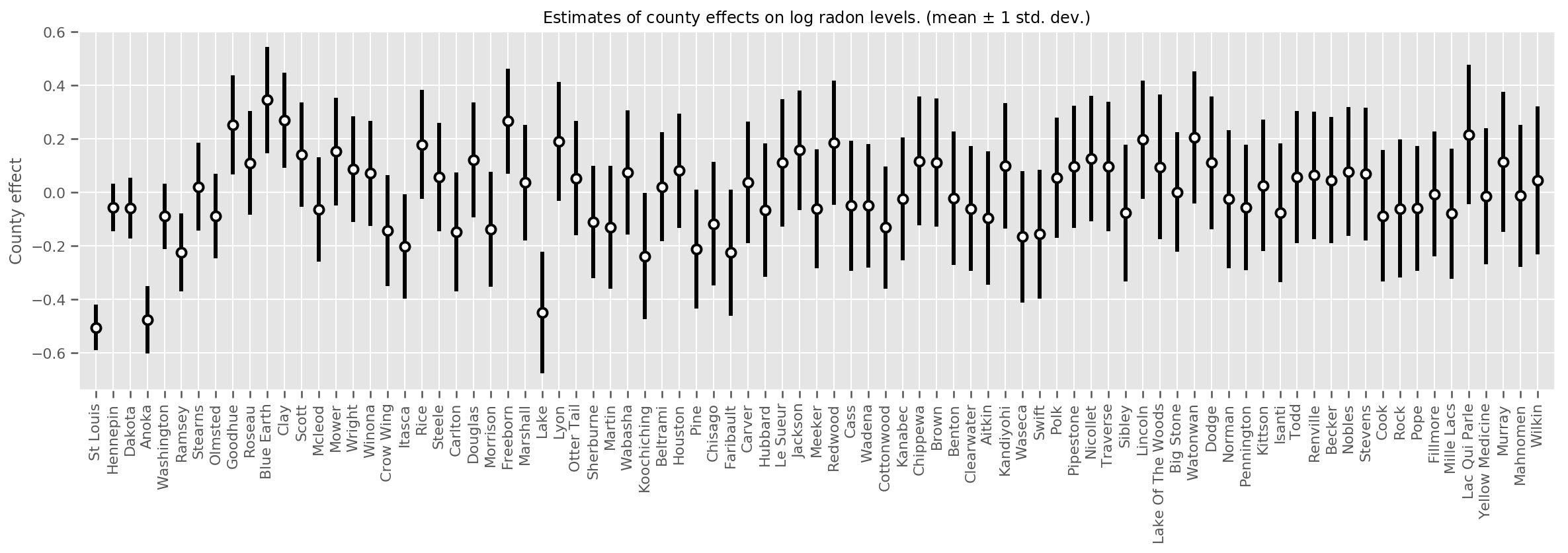
เราสามารถพลอตผลกระทบของค่าเฉลี่ยเคาน์ตี ร่วมกับความไม่แน่นอนของค่าเฉลี่ยนั้นได้ เราได้เรียงลำดับตามจำนวนการสังเกต โดยขนาดใหญ่ที่สุดอยู่ทางซ้าย สังเกตว่าความไม่แน่นอนมีน้อยสำหรับมณฑลที่มีข้อสังเกตมากมาย แต่จะมีมากขึ้นสำหรับมณฑลที่มีข้อสังเกตเพียงหนึ่งหรือสองแห่ง
county_counts = (df.groupby(by=['county', 'county_code'], observed=True)
                   .agg('size')
                   .sort_values(ascending=False)
                   .reset_index(name='count'))

means = county_weights_.mean()
stds = county_weights_.stddev()

fig, ax = plt.subplots(figsize=(20, 5))

for idx, row in county_counts.iterrows():
  mid = means[row.county_code]
  std = stds[row.county_code]
  ax.vlines(idx, mid - std, mid + std, linewidth=3)
  ax.plot(idx, means[row.county_code], 'ko', mfc='w', mew=2, ms=7)

ax.set(
    xticks=np.arange(len(county_counts)),
    xlim=(-1, len(county_counts)),
    ylabel="County effect",
    title=r"Estimates of county effects on log radon levels. (mean $\pm$ 1 std. dev.)",
)
ax.set_xticklabels(county_counts.county, rotation=90);
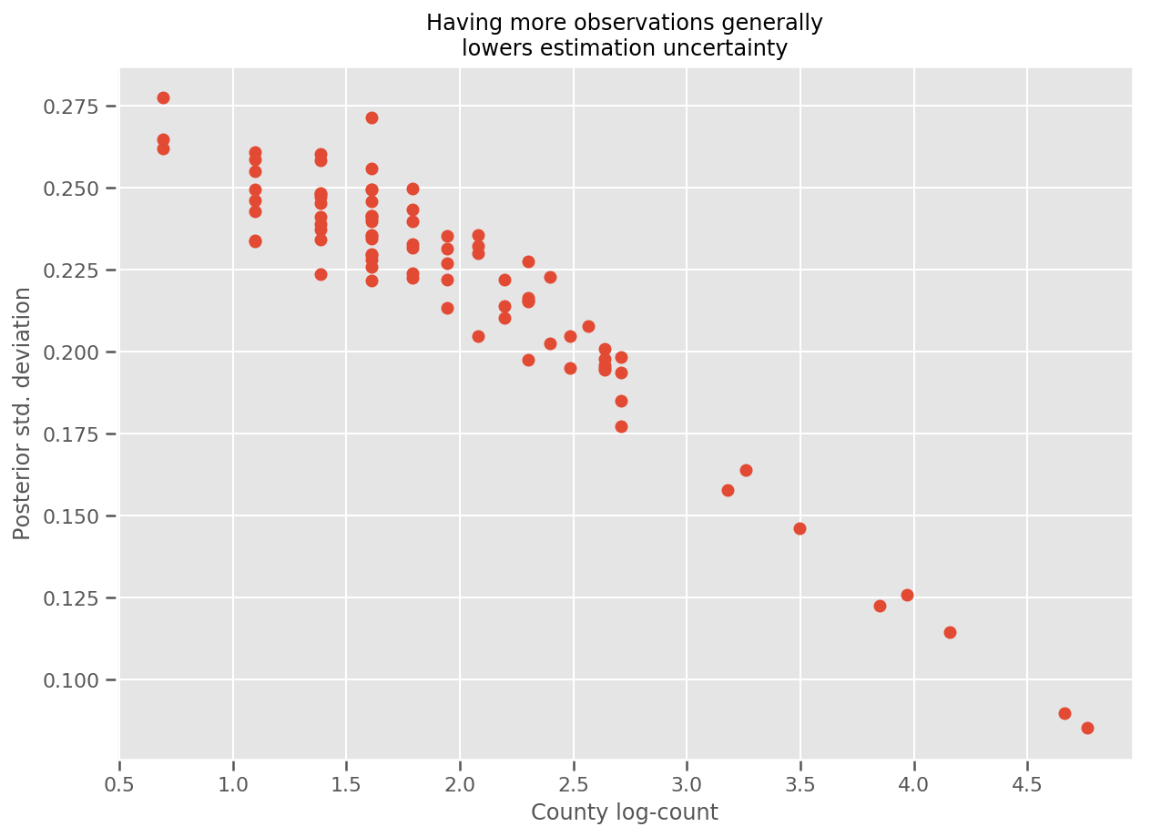
ที่จริงแล้ว เราสามารถเห็นสิ่งนี้ได้โดยตรงมากขึ้นโดยพล็อตจำนวนบันทึกของการสังเกตเทียบกับค่าเบี่ยงเบนมาตรฐานโดยประมาณ และดูความสัมพันธ์เป็นเส้นตรงโดยประมาณ
fig, ax = plt.subplots(figsize=(10, 7))
ax.plot(np.log1p(county_counts['count']), stds.numpy()[county_counts.county_code], 'o')
ax.set(
    ylabel='Posterior std. deviation',
    xlabel='County log-count',
    title='Having more observations generally\nlowers estimation uncertainty'
);
เมื่อเปรียบเทียบกับ lme4 ใน R
%%shell
exit  # Trick to make this block not execute.

radon = read.csv('srrs2.dat', header = TRUE)
radon = radon[radon$state=='MN',]
radon$radon = ifelse(radon$activity==0., 0.1, radon$activity)
radon$log_radon = log(radon$radon)

# install.packages('lme4')
library(lme4)
fit <- lmer(log_radon ~ 1 + floor + (1 | county), data=radon)
fit

# Linear mixed model fit by REML ['lmerMod']
# Formula: log_radon ~ 1 + floor + (1 | county)
#    Data: radon
# REML criterion at convergence: 2171.305
# Random effects:
#  Groups   Name        Std.Dev.
#  county   (Intercept) 0.3282
#  Residual             0.7556
# Number of obs: 919, groups:  county, 85
# Fixed Effects:
# (Intercept)        floor
#       1.462       -0.693
<IPython.core.display.Javascript at 0x7f90b888e9b0>
<IPython.core.display.Javascript at 0x7f90b888e780>
<IPython.core.display.Javascript at 0x7f90b888e780>
<IPython.core.display.Javascript at 0x7f90bce1dfd0>
<IPython.core.display.Javascript at 0x7f90b888e780>
<IPython.core.display.Javascript at 0x7f90b888e780>
<IPython.core.display.Javascript at 0x7f90b888e780>
<IPython.core.display.Javascript at 0x7f90b888e780>
ตารางต่อไปนี้สรุปผลลัพธ์
print(pd.DataFrame(data=dict(intercept=[1.462, tf.reduce_mean(intercept_.mean()).numpy()],
                             floor=[-0.693, tf.reduce_mean(floor_weight_.mean()).numpy()],
                             scale=[0.3282, tf.reduce_mean(scale_prior_.sample(10000)).numpy()]),
                   index=['lme4', 'vi']))
intercept   floor     scale
lme4   1.462000 -0.6930  0.328200
vi     1.435284 -0.6702  0.287251
ตารางนี้จะแสดงให้เห็นผลที่หกอยู่ภายใน ~ 10% ของ lme4 's ค่อนข้างน่าแปลกใจเพราะ:
-
lme4จะขึ้นอยู่กับ วิธีการเลซ (ไม่ใช่ VI) - colab นี้ไม่ได้พยายามมาบรรจบกันจริงๆ
- มีความพยายามน้อยที่สุดในการปรับแต่งไฮเปอร์พารามิเตอร์
- ไม่มีความพยายามใด ๆ ที่จะทำให้ข้อมูลเป็นปกติหรือประมวลผลล่วงหน้า (เช่น คุณสมบัติศูนย์ ฯลฯ)
บทสรุป
ใน colab นี้ เราได้อธิบายเกี่ยวกับ Generalized Linear Mixed-Effects Models และแสดงวิธีใช้การอนุมานแบบแปรผันเพื่อให้เข้ากับมันโดยใช้ความน่าจะเป็นของ TensorFlow แม้ว่าปัญหาของเล่นจะมีตัวอย่างการฝึกเพียงไม่กี่ร้อยตัวอย่าง แต่เทคนิคที่ใช้ในที่นี้ก็เหมือนกับที่ต้องการในปริมาณมาก