
| | |  ดูแหล่งที่มาบน GitHub ดูแหล่งที่มาบน GitHub | |
ความน่าจะเป็นการวิเคราะห์องค์ประกอบหลัก (PCA) เป็นเทคนิคการลดมิติที่ช่วยวิเคราะห์ข้อมูลผ่านพื้นที่แฝงมิติที่ต่ำกว่า ( Tipping และบิชอป 1999 ) มักใช้เมื่อมีค่าที่ขาดหายไปในข้อมูลหรือสำหรับการปรับขนาดหลายมิติ
นำเข้า
import functools
import warnings

import matplotlib.pyplot as plt
import numpy as np
import seaborn as sns

import tensorflow.compat.v2 as tf
import tensorflow_probability as tfp

from tensorflow_probability import bijectors as tfb
from tensorflow_probability import distributions as tfd

tf.enable_v2_behavior()

plt.style.use("ggplot")
warnings.filterwarnings('ignore')
นางแบบ
พิจารณาข้อมูลชุด \(\mathbf{X} = \{\mathbf{x}_n\}\) ของ \(N\) จุดข้อมูลที่แต่ละจุดข้อมูลเป็น \(D\)มิติ, $ \ mathbf {x} _n \ in \ mathbb {R} ^ D\(. We aim to represent each \)\ mathbf {x} _n ภายใต้ $ ตัวแปรแฝง \(\mathbf{z}_n \in \mathbb{R}^K\) กับมิติที่ต่ำกว่า $ K <D\(. The set of principal axes \)\ mathbf {W} $ เกี่ยวข้องตัวแปรแฝงข้อมูล
โดยเฉพาะอย่างยิ่ง เราคิดว่าตัวแปรแฝงแต่ละตัวมีการกระจายตามปกติ
\[ \begin{equation*} \mathbf{z}_n \sim N(\mathbf{0}, \mathbf{I}). \end{equation*} \]
จุดข้อมูลที่สอดคล้องกันถูกสร้างขึ้นผ่านการฉายภาพ
\[ \begin{equation*} \mathbf{x}_n \mid \mathbf{z}_n \sim N(\mathbf{W}\mathbf{z}_n, \sigma^2\mathbf{I}), \end{equation*} \]
ที่เมทริกซ์ \(\mathbf{W}\in\mathbb{R}^{D\times K}\) เป็นที่รู้จักกันเป็นแกนหลัก ใน PCA น่าจะเป็นเรามักจะมีความสนใจในการประมาณแกนหลัก \(\mathbf{W}\) และระยะเสียง\(\sigma^2\)
PCA ความน่าจะเป็นโดยทั่วไป PCA แบบคลาสสิก การหาระยะขอบของตัวแปรแฝง การกระจายของจุดข้อมูลแต่ละจุดคือ
\[ \begin{equation*} \mathbf{x}_n \sim N(\mathbf{0}, \mathbf{W}\mathbf{W}^\top + \sigma^2\mathbf{I}). \end{equation*} \]
PCA คลาสสิกเป็นกรณีที่เฉพาะเจาะจงของ PCA น่าจะเป็นเมื่อความแปรปรวนของเสียงจะกลายเป็นขนาดเล็กกระจิริด \(\sigma^2 \to 0\)
เราตั้งค่าโมเดลของเราด้านล่าง ในการวิเคราะห์ของเราเราถือว่า \(\sigma\) เป็นที่รู้จักกันและแทนการจุดประมาณ \(\mathbf{W}\) เป็นพารามิเตอร์รุ่นเราวางก่อนที่มากกว่านั้นเพื่อที่จะสรุปการจัดจำหน่ายมากกว่าแกนหลัก เราจะแสดงรูปแบบเป็น TFP JointDistribution เฉพาะเราจะใช้ JointDistributionCoroutineAutoBatched
def probabilistic_pca(data_dim, latent_dim, num_datapoints, stddv_datapoints):
  w = yield tfd.Normal(loc=tf.zeros([data_dim, latent_dim]),
                 scale=2.0 * tf.ones([data_dim, latent_dim]),
                 name="w")
  z = yield tfd.Normal(loc=tf.zeros([latent_dim, num_datapoints]),
                 scale=tf.ones([latent_dim, num_datapoints]),
                 name="z")
  x = yield tfd.Normal(loc=tf.matmul(w, z),
                       scale=stddv_datapoints,
                       name="x")
num_datapoints = 5000
data_dim = 2
latent_dim = 1
stddv_datapoints = 0.5

concrete_ppca_model = functools.partial(probabilistic_pca,
    data_dim=data_dim,
    latent_dim=latent_dim,
    num_datapoints=num_datapoints,
    stddv_datapoints=stddv_datapoints)

model = tfd.JointDistributionCoroutineAutoBatched(concrete_ppca_model)
ข้อมูล
เราสามารถใช้แบบจำลองเพื่อสร้างข้อมูลโดยการสุ่มตัวอย่างจากการแจกแจงร่วมกันก่อน
actual_w, actual_z, x_train = model.sample()

print("Principal axes:")
print(actual_w)
Principal axes:
tf.Tensor(
[[ 2.2801023]
 [-1.1619819]], shape=(2, 1), dtype=float32)
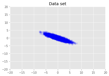
เราเห็นภาพชุดข้อมูล
plt.scatter(x_train[0, :], x_train[1, :], color='blue', alpha=0.1)
plt.axis([-20, 20, -20, 20])
plt.title("Data set")
plt.show()
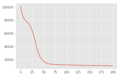
การอนุมาน Posteriori สูงสุด
ก่อนอื่นเราค้นหาการประมาณค่าจุดของตัวแปรแฝงที่เพิ่มความหนาแน่นของความน่าจะเป็นภายหลังสูงสุด นี้เป็นที่รู้จักกันเป็นสูงสุด posteriori (MAP) การอนุมานและจะทำโดยการคำนวณค่าของ \(\mathbf{W}\) และ \(\mathbf{Z}\) ที่เพิ่มความหนาแน่นหลัง \(p(\mathbf{W}, \mathbf{Z} \mid \mathbf{X}) \propto p(\mathbf{W}, \mathbf{Z}, \mathbf{X})\)
w = tf.Variable(tf.random.normal([data_dim, latent_dim]))
z = tf.Variable(tf.random.normal([latent_dim, num_datapoints]))

target_log_prob_fn = lambda w, z: model.log_prob((w, z, x_train))
losses = tfp.math.minimize(
    lambda: -target_log_prob_fn(w, z),
    optimizer=tf.optimizers.Adam(learning_rate=0.05),
    num_steps=200)
plt.plot(losses)
[<matplotlib.lines.Line2D at 0x7f19897a42e8>]
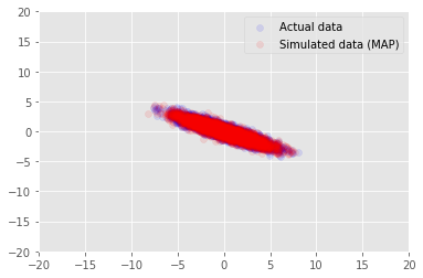
เราสามารถใช้แบบจำลองเพื่อใช้ข้อมูลตัวอย่างสำหรับค่าอนุมานสำหรับ \(\mathbf{W}\) และ \(\mathbf{Z}\)และเปรียบเทียบกับชุดข้อมูลที่เกิดขึ้นจริงเราปรับอากาศบน
print("MAP-estimated axes:")
print(w)

_, _, x_generated = model.sample(value=(w, z, None))

plt.scatter(x_train[0, :], x_train[1, :], color='blue', alpha=0.1, label='Actual data')
plt.scatter(x_generated[0, :], x_generated[1, :], color='red', alpha=0.1, label='Simulated data (MAP)')
plt.legend()
plt.axis([-20, 20, -20, 20])
plt.show()
MAP-estimated axes:
<tf.Variable 'Variable:0' shape=(2, 1) dtype=float32, numpy=
array([[ 2.9135954],
       [-1.4826864]], dtype=float32)>
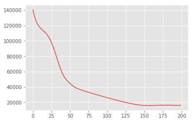
การอนุมานแบบแปรผัน
MAP สามารถใช้เพื่อค้นหาโหมด (หรือโหมดใดโหมดหนึ่ง) ของการแจกแจงภายหลัง แต่ไม่ได้ให้ข้อมูลเชิงลึกอื่นๆ เกี่ยวกับโหมดนี้ ต่อไปเราจะใช้การอนุมานแปรผันที่หลัง Distribtion \(p(\mathbf{W}, \mathbf{Z} \mid \mathbf{X})\) เป็นห้วงใช้การกระจายแปรผัน \(q(\mathbf{W}, \mathbf{Z})\) parametrised โดย \(\boldsymbol{\lambda}\)จุดมุ่งหมายคือการหาพารามิเตอร์แปรผัน \(\boldsymbol{\lambda}\) ที่ลดความแตกต่างระหว่าง KL Q และหลัง, \(\mathrm{KL}(q(\mathbf{W}, \mathbf{Z}) \mid\mid p(\mathbf{W}, \mathbf{Z} \mid \mathbf{X}))\)หรือเท่าที่เพิ่มหลักฐานที่ต่ำกว่าผูกพัน \(\mathbb{E}_{q(\mathbf{W},\mathbf{Z};\boldsymbol{\lambda})}\left[ \log p(\mathbf{W},\mathbf{Z},\mathbf{X}) - \log q(\mathbf{W},\mathbf{Z}; \boldsymbol{\lambda}) \right]\)
qw_mean = tf.Variable(tf.random.normal([data_dim, latent_dim]))
qz_mean = tf.Variable(tf.random.normal([latent_dim, num_datapoints]))
qw_stddv = tfp.util.TransformedVariable(1e-4 * tf.ones([data_dim, latent_dim]),
                                        bijector=tfb.Softplus())
qz_stddv = tfp.util.TransformedVariable(
    1e-4 * tf.ones([latent_dim, num_datapoints]),
    bijector=tfb.Softplus())
def factored_normal_variational_model():
  qw = yield tfd.Normal(loc=qw_mean, scale=qw_stddv, name="qw")
  qz = yield tfd.Normal(loc=qz_mean, scale=qz_stddv, name="qz")

surrogate_posterior = tfd.JointDistributionCoroutineAutoBatched(
    factored_normal_variational_model)

losses = tfp.vi.fit_surrogate_posterior(
    target_log_prob_fn,
    surrogate_posterior=surrogate_posterior,
    optimizer=tf.optimizers.Adam(learning_rate=0.05),
    num_steps=200)
print("Inferred axes:")
print(qw_mean)
print("Standard Deviation:")
print(qw_stddv)

plt.plot(losses)
plt.show()
Inferred axes:
<tf.Variable 'Variable:0' shape=(2, 1) dtype=float32, numpy=
array([[ 2.4168603],
       [-1.2236133]], dtype=float32)>
Standard Deviation:
<TransformedVariable: dtype=float32, shape=[2, 1], fn="softplus", numpy=
array([[0.0042499 ],
       [0.00598824]], dtype=float32)>
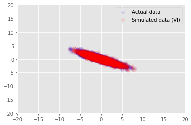
posterior_samples = surrogate_posterior.sample(50)
_, _, x_generated = model.sample(value=(posterior_samples))

# It's a pain to plot all 5000 points for each of our 50 posterior samples, so
# let's subsample to get the gist of the distribution.
x_generated = tf.reshape(tf.transpose(x_generated, [1, 0, 2]), (2, -1))[:, ::47]

plt.scatter(x_train[0, :], x_train[1, :], color='blue', alpha=0.1, label='Actual data')
plt.scatter(x_generated[0, :], x_generated[1, :], color='red', alpha=0.1, label='Simulated data (VI)')
plt.legend()
plt.axis([-20, 20, -20, 20])
plt.show()
รับทราบ
กวดวิชานี้ถูกเขียนเดิมในเอ็ดเวิร์ด 1.0 ( แหล่งที่มา ) เราขอขอบคุณผู้ร่วมเขียนข้อความและแก้ไขเวอร์ชันนั้น
อ้างอิง
[1]: Michael E. Tipping และ Christopher M. Bishop การวิเคราะห์องค์ประกอบหลักความน่าจะเป็น วารสารของสมาคมสถิติ: Series B (วิธีการทางสถิติ), 61 (3): 611-622 1999