สมุดบันทึกนี้แสดงตัวอย่างสองตัวอย่างของแบบจำลองอนุกรมเวลาเชิงโครงสร้างที่เหมาะสมกับอนุกรมเวลา และใช้แบบจำลองเหล่านี้เพื่อสร้างการคาดการณ์และคำอธิบาย
| | |  ดูแหล่งที่มาบน GitHub ดูแหล่งที่มาบน GitHub | |
การพึ่งพาและข้อกำหนดเบื้องต้น
นำเข้าและตั้งค่า
%matplotlib inline
import matplotlib as mpl
from matplotlib import pylab as plt
import matplotlib.dates as mdates
import seaborn as sns

import collections

import numpy as np
import tensorflow.compat.v2 as tf
import tensorflow_probability as tfp

from tensorflow_probability import distributions as tfd
from tensorflow_probability import sts

tf.enable_v2_behavior()
ทำสิ่งที่รวดเร็ว!
ก่อนที่เราจะเจาะลึก มาทำให้มั่นใจว่าเรากำลังใช้ GPU สำหรับการสาธิตนี้
ในการดำเนินการนี้ ให้เลือก "รันไทม์" -> "เปลี่ยนประเภทรันไทม์" -> "ตัวเร่งฮาร์ดแวร์" -> "GPU"
ตัวอย่างต่อไปนี้จะตรวจสอบว่าเรามีสิทธิ์เข้าถึง GPU
if tf.test.gpu_device_name() != '/device:GPU:0':
  print('WARNING: GPU device not found.')
else:
  print('SUCCESS: Found GPU: {}'.format(tf.test.gpu_device_name()))
SUCCESS: Found GPU: /device:GPU:0
การตั้งค่าพล็อต
เมธอดตัวช่วยสำหรับพล็อตอนุกรมเวลาและการคาดการณ์
from pandas.plotting import register_matplotlib_converters
register_matplotlib_converters()

sns.set_context("notebook", font_scale=1.)
sns.set_style("whitegrid")
%config InlineBackend.figure_format = 'retina'
def plot_forecast(x, y,
                  forecast_mean, forecast_scale, forecast_samples,
                  title, x_locator=None, x_formatter=None):
  """Plot a forecast distribution against the 'true' time series."""
  colors = sns.color_palette()
  c1, c2 = colors[0], colors[1]
  fig = plt.figure(figsize=(12, 6))
  ax = fig.add_subplot(1, 1, 1)

  num_steps = len(y)
  num_steps_forecast = forecast_mean.shape[-1]
  num_steps_train = num_steps - num_steps_forecast


  ax.plot(x, y, lw=2, color=c1, label='ground truth')

  forecast_steps = np.arange(
      x[num_steps_train],
      x[num_steps_train]+num_steps_forecast,
      dtype=x.dtype)

  ax.plot(forecast_steps, forecast_samples.T, lw=1, color=c2, alpha=0.1)

  ax.plot(forecast_steps, forecast_mean, lw=2, ls='--', color=c2,
           label='forecast')
  ax.fill_between(forecast_steps,
                   forecast_mean-2*forecast_scale,
                   forecast_mean+2*forecast_scale, color=c2, alpha=0.2)

  ymin, ymax = min(np.min(forecast_samples), np.min(y)), max(np.max(forecast_samples), np.max(y))
  yrange = ymax-ymin
  ax.set_ylim([ymin - yrange*0.1, ymax + yrange*0.1])
  ax.set_title("{}".format(title))
  ax.legend()

  if x_locator is not None:
    ax.xaxis.set_major_locator(x_locator)
    ax.xaxis.set_major_formatter(x_formatter)
    fig.autofmt_xdate()

  return fig, ax
def plot_components(dates,
                    component_means_dict,
                    component_stddevs_dict,
                    x_locator=None,
                    x_formatter=None):
  """Plot the contributions of posterior components in a single figure."""
  colors = sns.color_palette()
  c1, c2 = colors[0], colors[1]

  axes_dict = collections.OrderedDict()
  num_components = len(component_means_dict)
  fig = plt.figure(figsize=(12, 2.5 * num_components))
  for i, component_name in enumerate(component_means_dict.keys()):
    component_mean = component_means_dict[component_name]
    component_stddev = component_stddevs_dict[component_name]

    ax = fig.add_subplot(num_components,1,1+i)
    ax.plot(dates, component_mean, lw=2)
    ax.fill_between(dates,
                     component_mean-2*component_stddev,
                     component_mean+2*component_stddev,
                     color=c2, alpha=0.5)
    ax.set_title(component_name)
    if x_locator is not None:
      ax.xaxis.set_major_locator(x_locator)
      ax.xaxis.set_major_formatter(x_formatter)
    axes_dict[component_name] = ax
  fig.autofmt_xdate()
  fig.tight_layout()
  return fig, axes_dict
def plot_one_step_predictive(dates, observed_time_series,
                             one_step_mean, one_step_scale,
                             x_locator=None, x_formatter=None):
  """Plot a time series against a model's one-step predictions."""

  colors = sns.color_palette()
  c1, c2 = colors[0], colors[1]

  fig=plt.figure(figsize=(12, 6))
  ax = fig.add_subplot(1,1,1)
  num_timesteps = one_step_mean.shape[-1]
  ax.plot(dates, observed_time_series, label="observed time series", color=c1)
  ax.plot(dates, one_step_mean, label="one-step prediction", color=c2)
  ax.fill_between(dates,
                  one_step_mean - one_step_scale,
                  one_step_mean + one_step_scale,
                  alpha=0.1, color=c2)
  ax.legend()

  if x_locator is not None:
    ax.xaxis.set_major_locator(x_locator)
    ax.xaxis.set_major_formatter(x_formatter)
    fig.autofmt_xdate()
  fig.tight_layout()
  return fig, ax
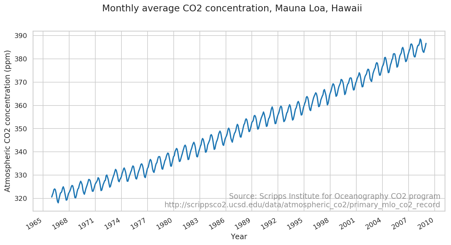
บันทึก Mauna Loa CO2
เราจะสาธิตการปรับแบบจำลองให้เหมาะสมกับการอ่านค่า CO2 ในบรรยากาศจากหอสังเกตการณ์ Mauna Loa
ข้อมูล
# CO2 readings from Mauna Loa observatory, monthly beginning January 1966
# Original source: http://scrippsco2.ucsd.edu/data/atmospheric_co2/primary_mlo_co2_record
co2_by_month = np.array('320.62,321.60,322.39,323.70,324.08,323.75,322.38,320.36,318.64,318.10,319.78,321.03,322.33,322.50,323.04,324.42,325.00,324.09,322.54,320.92,319.25,319.39,320.73,321.96,322.57,323.15,323.89,325.02,325.57,325.36,324.14,322.11,320.33,320.25,321.32,322.89,324.00,324.42,325.63,326.66,327.38,326.71,325.88,323.66,322.38,321.78,322.85,324.12,325.06,325.98,326.93,328.14,328.08,327.67,326.34,324.69,323.10,323.06,324.01,325.13,326.17,326.68,327.17,327.79,328.92,328.57,327.36,325.43,323.36,323.56,324.80,326.01,326.77,327.63,327.75,329.73,330.07,329.09,328.04,326.32,324.84,325.20,326.50,327.55,328.55,329.56,330.30,331.50,332.48,332.07,330.87,329.31,327.51,327.18,328.16,328.64,329.35,330.71,331.48,332.65,333.09,332.25,331.18,329.39,327.43,327.37,328.46,329.57,330.40,331.40,332.04,333.31,333.97,333.60,331.90,330.06,328.56,328.34,329.49,330.76,331.75,332.56,333.50,334.58,334.88,334.33,333.05,330.94,329.30,328.94,330.31,331.68,332.93,333.42,334.70,336.07,336.75,336.27,334.92,332.75,331.59,331.16,332.40,333.85,334.97,335.38,336.64,337.76,338.01,337.89,336.54,334.68,332.76,332.55,333.92,334.95,336.23,336.76,337.96,338.88,339.47,339.29,337.73,336.09,333.92,333.86,335.29,336.73,338.01,338.36,340.07,340.77,341.47,341.17,339.56,337.60,335.88,336.02,337.10,338.21,339.24,340.48,341.38,342.51,342.91,342.25,340.49,338.43,336.69,336.86,338.36,339.61,340.75,341.61,342.70,343.57,344.14,343.35,342.06,339.81,337.98,337.86,339.26,340.49,341.38,342.52,343.10,344.94,345.76,345.32,343.98,342.38,339.87,339.99,341.15,342.99,343.70,344.50,345.28,347.06,347.43,346.80,345.39,343.28,341.07,341.35,342.98,344.22,344.97,345.99,347.42,348.35,348.93,348.25,346.56,344.67,343.09,342.80,344.24,345.56,346.30,346.95,347.85,349.55,350.21,349.55,347.94,345.90,344.85,344.17,345.66,346.90,348.02,348.48,349.42,350.99,351.85,351.26,349.51,348.10,346.45,346.36,347.81,348.96,350.43,351.73,352.22,353.59,354.22,353.79,352.38,350.43,348.73,348.88,350.07,351.34,352.76,353.07,353.68,355.42,355.67,355.12,353.90,351.67,349.80,349.99,351.30,352.52,353.66,354.70,355.38,356.20,357.16,356.23,354.81,352.91,350.96,351.18,352.83,354.21,354.72,355.75,357.16,358.60,359.34,358.24,356.17,354.02,352.15,352.21,353.75,354.99,355.99,356.72,357.81,359.15,359.66,359.25,357.02,355.00,353.01,353.31,354.16,355.40,356.70,357.17,358.38,359.46,360.28,359.60,357.57,355.52,353.69,353.99,355.34,356.80,358.37,358.91,359.97,361.26,361.69,360.94,359.55,357.48,355.84,356.00,357.58,359.04,359.97,361.00,361.64,363.45,363.80,363.26,361.89,359.45,358.05,357.75,359.56,360.70,362.05,363.24,364.02,364.71,365.41,364.97,363.65,361.48,359.45,359.61,360.76,362.33,363.18,363.99,364.56,366.36,366.80,365.63,364.47,362.50,360.19,360.78,362.43,364.28,365.33,366.15,367.31,368.61,369.30,368.88,367.64,365.78,363.90,364.23,365.46,366.97,368.15,368.87,369.59,371.14,371.00,370.35,369.27,366.93,364.64,365.13,366.68,368.00,369.14,369.46,370.51,371.66,371.83,371.69,370.12,368.12,366.62,366.73,368.29,369.53,370.28,371.50,372.12,372.86,374.02,373.31,371.62,369.55,367.96,368.09,369.68,371.24,372.44,373.08,373.52,374.85,375.55,375.40,374.02,371.48,370.70,370.25,372.08,373.78,374.68,375.62,376.11,377.65,378.35,378.13,376.61,374.48,372.98,373.00,374.35,375.69,376.79,377.36,378.39,380.50,380.62,379.55,377.76,375.83,374.05,374.22,375.84,377.44,378.34,379.61,380.08,382.05,382.24,382.08,380.67,378.67,376.42,376.80,378.31,379.96,381.37,382.02,382.56,384.37,384.92,384.03,382.28,380.48,378.81,379.06,380.14,381.66,382.58,383.71,384.34,386.23,386.41,385.87,384.45,381.84,380.86,380.86,382.36,383.61,385.07,385.84,385.83,386.77,388.51,388.05,386.25,384.08,383.09,382.78,384.01,385.11,386.65,387.12,388.52,389.57,390.16,389.62,388.07,386.08,384.65,384.33,386.05,387.49,388.55,390.07,391.01,392.38,393.22,392.24,390.33,388.52,386.84,387.16,388.67,389.81,391.30,391.92,392.45,393.37,394.28,393.69,392.59,390.21,389.00,388.93,390.24,391.80,393.07,393.35,394.36,396.43,396.87,395.88,394.52,392.54,391.13,391.01,392.95,394.34,395.61,396.85,397.26,398.35,399.98,398.87,397.37,395.41,393.39,393.70,395.19,396.82,397.92,398.10,399.47,401.33,401.88,401.31,399.07,397.21,395.40,395.65,397.23,398.79,399.85,400.31,401.51,403.45,404.10,402.88,401.61,399.00,397.50,398.28,400.24,401.89,402.65,404.16,404.85,407.57,407.66,407.00,404.50,402.24,401.01,401.50,403.64,404.55,406.07,406.64,407.06,408.95,409.91,409.12,407.20,405.24,403.27,403.64,405.17,406.75,408.05,408.34,409.25,410.30,411.30,410.88,408.90,407.10,405.59,405.99,408.12,409.23,410.92'.split(',')).astype(np.float32)

co2_by_month = co2_by_month
num_forecast_steps = 12 * 10 # Forecast the final ten years, given previous data
co2_by_month_training_data = co2_by_month[:-num_forecast_steps]

co2_dates = np.arange("1966-01", "2019-02", dtype="datetime64[M]")
co2_loc = mdates.YearLocator(3)
co2_fmt = mdates.DateFormatter('%Y')
fig = plt.figure(figsize=(12, 6))
ax = fig.add_subplot(1, 1, 1)
ax.plot(co2_dates[:-num_forecast_steps], co2_by_month_training_data, lw=2, label="training data")
ax.xaxis.set_major_locator(co2_loc)
ax.xaxis.set_major_formatter(co2_fmt)
ax.set_ylabel("Atmospheric CO2 concentration (ppm)")
ax.set_xlabel("Year")
fig.suptitle("Monthly average CO2 concentration, Mauna Loa, Hawaii",
             fontsize=15)
ax.text(0.99, .02,
        "Source: Scripps Institute for Oceanography CO2 program\nhttp://scrippsco2.ucsd.edu/data/atmospheric_co2/primary_mlo_co2_record",
        transform=ax.transAxes,
        horizontalalignment="right",
        alpha=0.5)
fig.autofmt_xdate()
รุ่นและฟิตติ้ง
เราจะสร้างแบบจำลองชุดนี้ด้วยแนวโน้มเชิงเส้นในท้องถิ่น บวกกับผลกระทบตามฤดูกาลในแต่ละเดือนของปี
def build_model(observed_time_series):
  trend = sts.LocalLinearTrend(observed_time_series=observed_time_series)
  seasonal = tfp.sts.Seasonal(
      num_seasons=12, observed_time_series=observed_time_series)
  model = sts.Sum([trend, seasonal], observed_time_series=observed_time_series)
  return model
เราจะปรับโมเดลโดยใช้การอนุมานแบบแปรผัน สิ่งนี้เกี่ยวข้องกับการเรียกใช้ตัวเพิ่มประสิทธิภาพเพื่อลดฟังก์ชันการสูญเสียที่แปรผัน หลักฐานเชิงลบขอบเขตล่าง (ELBO) เหมาะกับชุดของการแจกแจงหลังโดยประมาณสำหรับพารามิเตอร์ (ในทางปฏิบัติ เราถือว่าสิ่งเหล่านี้เป็นค่าปกติที่แปลงเป็นพื้นที่สนับสนุนของแต่ละพารามิเตอร์)
วิธีการพยากรณ์ tfp.sts ต้องใช้ตัวอย่างหลังเป็นอินพุต ดังนั้นเราจะเสร็จสิ้นโดยการวาดชุดของตัวอย่างจากส่วนหลังแบบแปรผัน
co2_model = build_model(co2_by_month_training_data)

# Build the variational surrogate posteriors `qs`.
variational_posteriors = tfp.sts.build_factored_surrogate_posterior(
    model=co2_model)
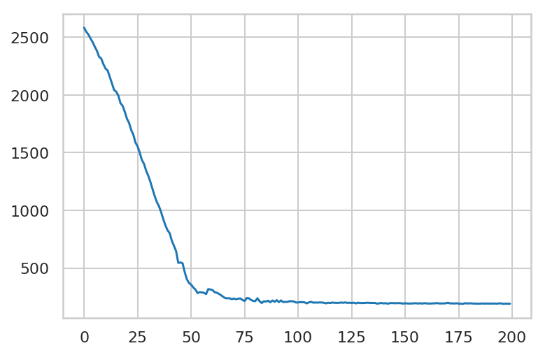
ลดการสูญเสียการแปรผันให้น้อยที่สุด
# Allow external control of optimization to reduce test runtimes.
num_variational_steps = 200 # @param { isTemplate: true}
num_variational_steps = int(num_variational_steps)

# Build and optimize the variational loss function.
elbo_loss_curve = tfp.vi.fit_surrogate_posterior(
    target_log_prob_fn=co2_model.joint_distribution(
        observed_time_series=co2_by_month_training_data).log_prob,
    surrogate_posterior=variational_posteriors,
    optimizer=tf.optimizers.Adam(learning_rate=0.1),
    num_steps=num_variational_steps,
    jit_compile=True)

plt.plot(elbo_loss_curve)
plt.show()

# Draw samples from the variational posterior.
q_samples_co2_ = variational_posteriors.sample(50)
WARNING:tensorflow:From /usr/local/lib/python3.6/dist-packages/tensorflow_core/python/ops/linalg/linear_operator_diag.py:166: calling LinearOperator.__init__ (from tensorflow.python.ops.linalg.linear_operator) with graph_parents is deprecated and will be removed in a future version.
Instructions for updating:
Do not pass `graph_parents`.  They will  no longer be used.
print("Inferred parameters:")
for param in co2_model.parameters:
  print("{}: {} +- {}".format(param.name,
                              np.mean(q_samples_co2_[param.name], axis=0),
                              np.std(q_samples_co2_[param.name], axis=0)))
Inferred parameters:
observation_noise_scale: 0.17199112474918365 +- 0.009443143382668495
LocalLinearTrend/_level_scale: 0.17671072483062744 +- 0.01510554924607277
LocalLinearTrend/_slope_scale: 0.004302256740629673 +- 0.0018349259626120329
Seasonal/_drift_scale: 0.041069451719522476 +- 0.007772190496325493
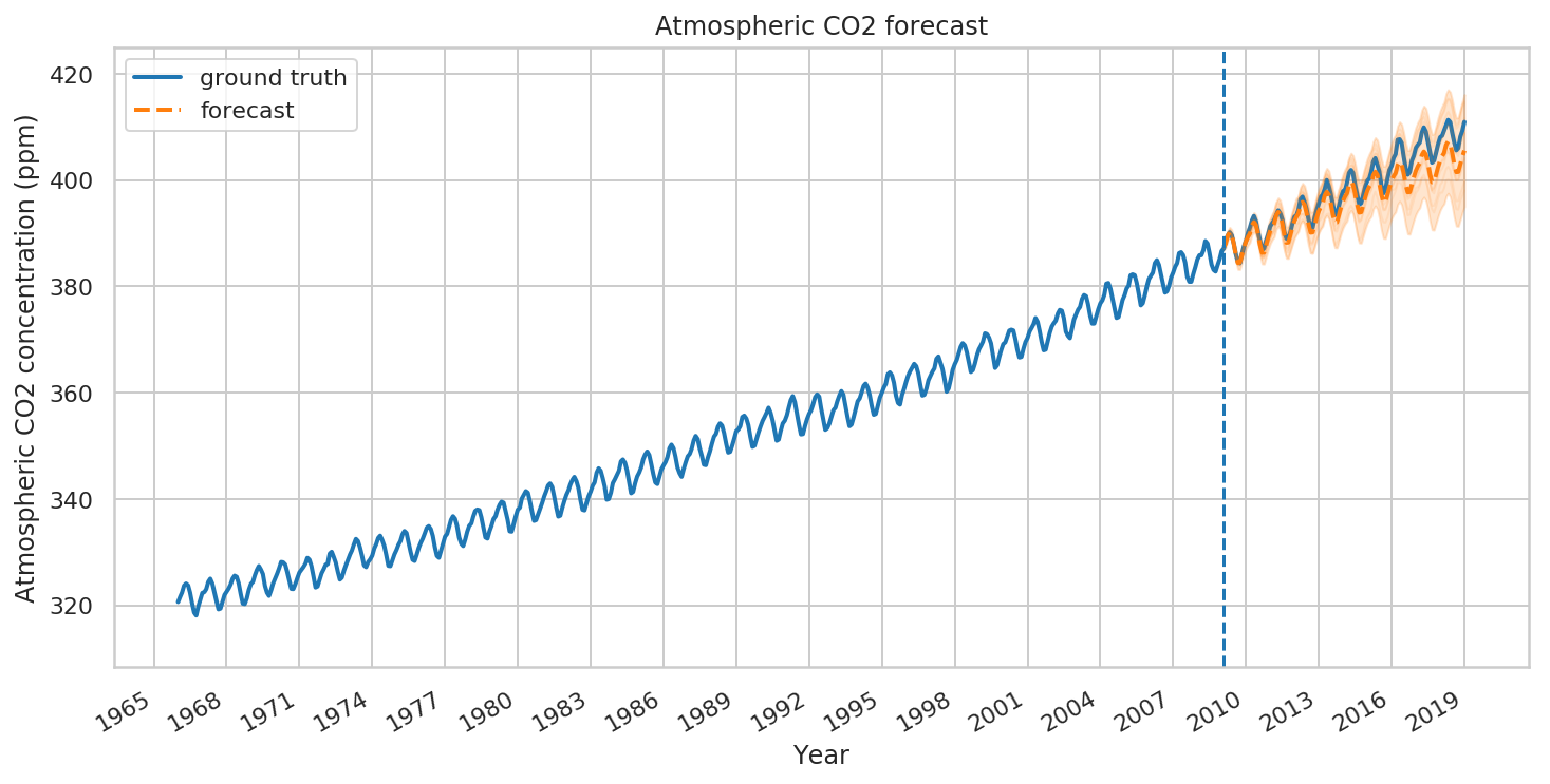
พยากรณ์และวิจารณ์
ตอนนี้ ลองใช้แบบจำลองที่พอดีเพื่อสร้างการคาดการณ์ เราเพียงแค่เรียก tfp.sts.forecast ซึ่งส่งคืนอินสแตนซ์ TensorFlow Distribution ที่แสดงถึงการกระจายเชิงคาดการณ์ในช่วงเวลาในอนาคต
co2_forecast_dist = tfp.sts.forecast(
    co2_model,
    observed_time_series=co2_by_month_training_data,
    parameter_samples=q_samples_co2_,
    num_steps_forecast=num_forecast_steps)
โดยเฉพาะอย่างยิ่ง mean และ stddev ของการกระจายการคาดการณ์ทำให้เราคาดการณ์ด้วยความไม่แน่นอนส่วนเพิ่มในแต่ละช่วงเวลา และเรายังสามารถวาดตัวอย่างของอนาคตที่เป็นไปได้อีกด้วย
num_samples=10

co2_forecast_mean, co2_forecast_scale, co2_forecast_samples = (
    co2_forecast_dist.mean().numpy()[..., 0],
    co2_forecast_dist.stddev().numpy()[..., 0],
    co2_forecast_dist.sample(num_samples).numpy()[..., 0])
fig, ax = plot_forecast(
    co2_dates, co2_by_month,
    co2_forecast_mean, co2_forecast_scale, co2_forecast_samples,
    x_locator=co2_loc,
    x_formatter=co2_fmt,
    title="Atmospheric CO2 forecast")
ax.axvline(co2_dates[-num_forecast_steps], linestyle="--")
ax.legend(loc="upper left")
ax.set_ylabel("Atmospheric CO2 concentration (ppm)")
ax.set_xlabel("Year")
fig.autofmt_xdate()
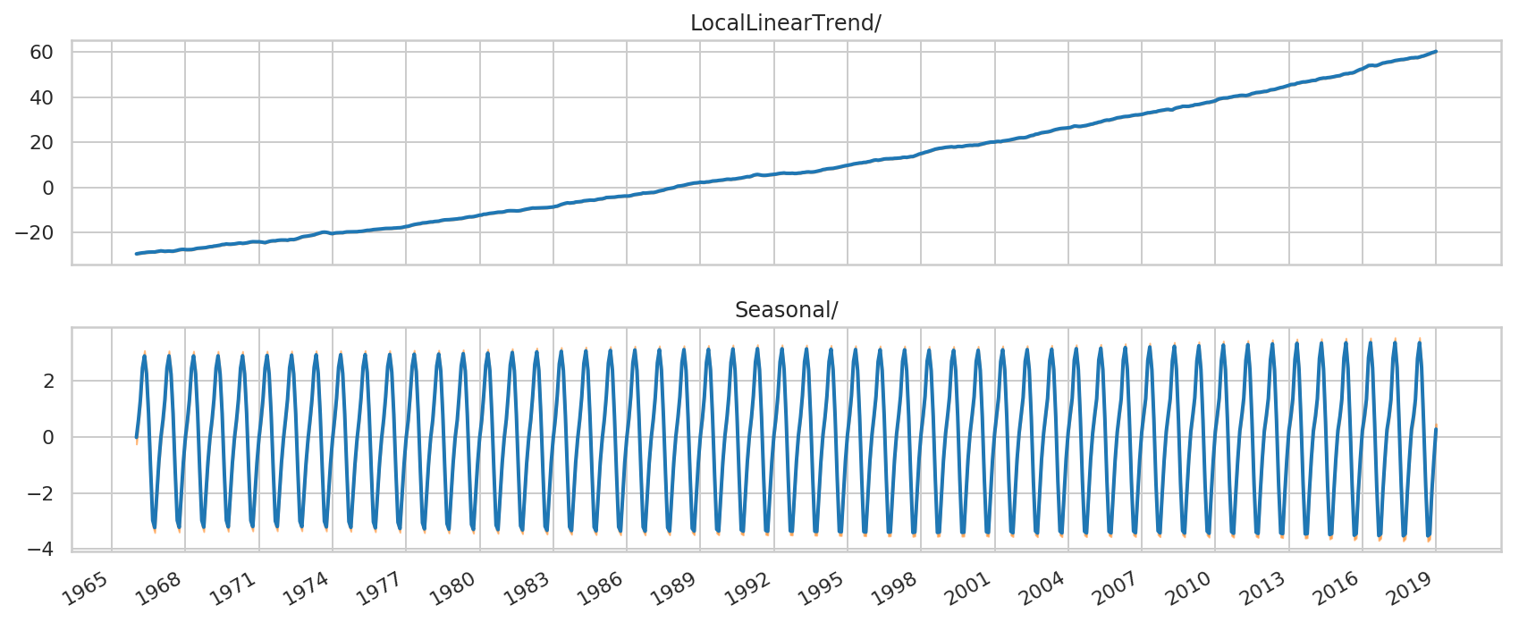
เราสามารถเข้าใจความพอดีของโมเดลเพิ่มเติมได้โดยการแยกย่อยเป็นส่วนร่วมของอนุกรมเวลาแต่ละแบบ:
# Build a dict mapping components to distributions over
# their contribution to the observed signal.
component_dists = sts.decompose_by_component(
    co2_model,
    observed_time_series=co2_by_month,
    parameter_samples=q_samples_co2_)
co2_component_means_, co2_component_stddevs_ = (
    {k.name: c.mean() for k, c in component_dists.items()},
    {k.name: c.stddev() for k, c in component_dists.items()})
_ = plot_components(co2_dates, co2_component_means_, co2_component_stddevs_,
                    x_locator=co2_loc, x_formatter=co2_fmt)
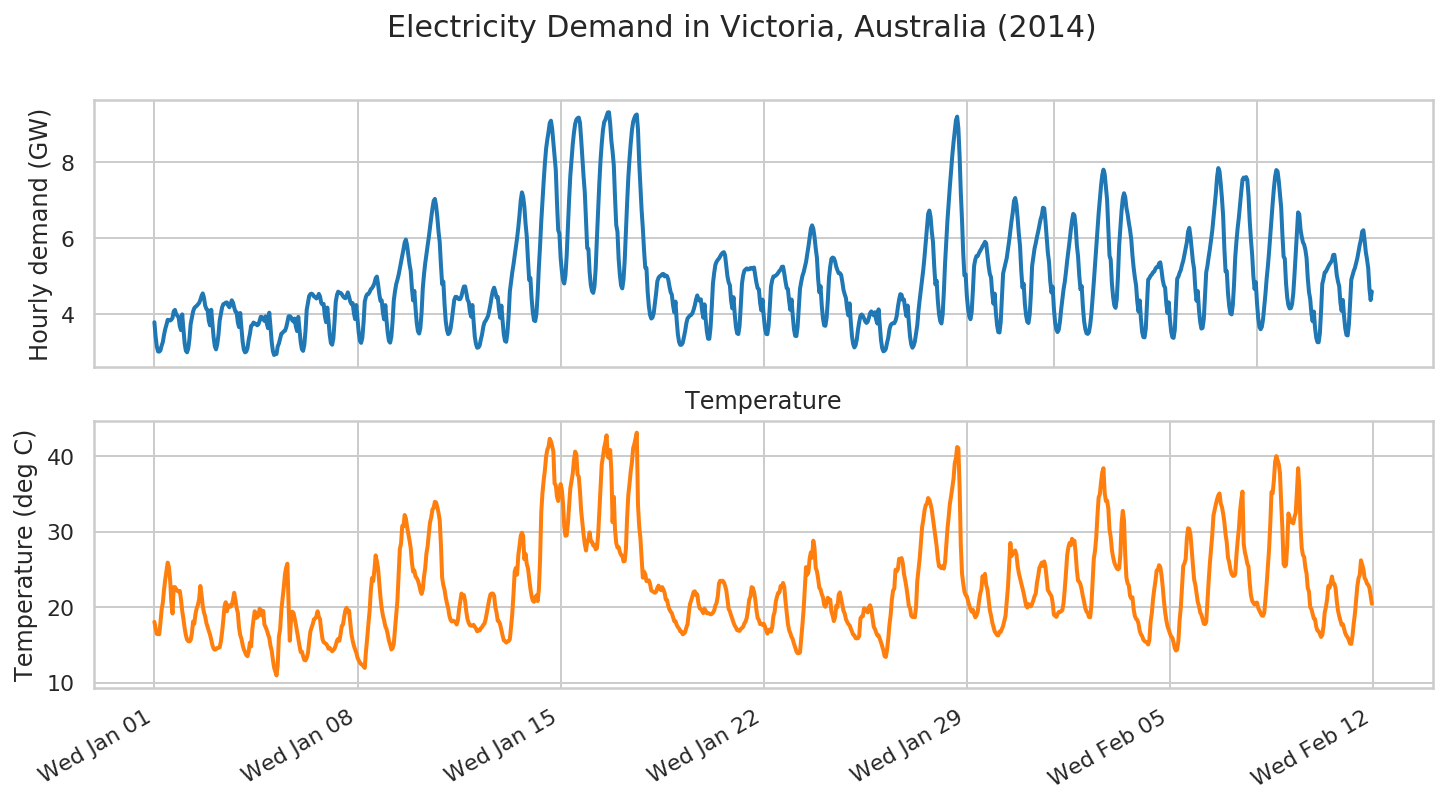
การพยากรณ์ความต้องการใช้ไฟฟ้า
ตอนนี้ มาลองพิจารณาตัวอย่างที่ซับซ้อนกว่านี้: การคาดการณ์ความต้องการไฟฟ้าในรัฐวิกตอเรีย ออสเตรเลีย
ขั้นแรก เราจะสร้างชุดข้อมูล:
# Victoria electricity demand dataset, as presented at
# https://otexts.com/fpp2/scatterplots.html
# and downloaded from https://github.com/robjhyndman/fpp2-package/blob/master/data/elecdaily.rda
# This series contains the first eight weeks (starting Jan 1). The original
# dataset was half-hourly data; here we've downsampled to hourly data by taking
# every other timestep.
demand_dates = np.arange('2014-01-01', '2014-02-26', dtype='datetime64[h]')
demand_loc = mdates.WeekdayLocator(byweekday=mdates.WE)
demand_fmt = mdates.DateFormatter('%a %b %d')

demand = np.array("3.794,3.418,3.152,3.026,3.022,3.055,3.180,3.276,3.467,3.620,3.730,3.858,3.851,3.839,3.861,3.912,4.082,4.118,4.011,3.965,3.932,3.693,3.585,4.001,3.623,3.249,3.047,3.004,3.104,3.361,3.749,3.910,4.075,4.165,4.202,4.225,4.265,4.301,4.381,4.484,4.552,4.440,4.233,4.145,4.116,3.831,3.712,4.121,3.764,3.394,3.159,3.081,3.216,3.468,3.838,4.012,4.183,4.269,4.280,4.310,4.315,4.233,4.188,4.263,4.370,4.308,4.182,4.075,4.057,3.791,3.667,4.036,3.636,3.283,3.073,3.003,3.023,3.113,3.335,3.484,3.697,3.723,3.786,3.763,3.748,3.714,3.737,3.828,3.937,3.929,3.877,3.829,3.950,3.756,3.638,4.045,3.682,3.283,3.036,2.933,2.956,2.959,3.157,3.236,3.370,3.493,3.516,3.555,3.570,3.656,3.792,3.950,3.953,3.926,3.849,3.813,3.891,3.683,3.562,3.936,3.602,3.271,3.085,3.041,3.201,3.570,4.123,4.307,4.481,4.533,4.545,4.524,4.470,4.457,4.418,4.453,4.539,4.473,4.301,4.260,4.276,3.958,3.796,4.180,3.843,3.465,3.246,3.203,3.360,3.808,4.328,4.509,4.598,4.562,4.566,4.532,4.477,4.442,4.424,4.486,4.579,4.466,4.338,4.270,4.296,4.034,3.877,4.246,3.883,3.520,3.306,3.252,3.387,3.784,4.335,4.465,4.529,4.536,4.589,4.660,4.691,4.747,4.819,4.950,4.994,4.798,4.540,4.352,4.370,4.047,3.870,4.245,3.848,3.509,3.302,3.258,3.419,3.809,4.363,4.605,4.793,4.908,5.040,5.204,5.358,5.538,5.708,5.888,5.966,5.817,5.571,5.321,5.141,4.686,4.367,4.618,4.158,3.771,3.555,3.497,3.646,4.053,4.687,5.052,5.342,5.586,5.808,6.038,6.296,6.548,6.787,6.982,7.035,6.855,6.561,6.181,5.899,5.304,4.795,4.862,4.264,3.820,3.588,3.481,3.514,3.632,3.857,4.116,4.375,4.462,4.460,4.422,4.398,4.407,4.480,4.621,4.732,4.735,4.572,4.385,4.323,4.069,3.940,4.247,3.821,3.416,3.220,3.124,3.132,3.181,3.337,3.469,3.668,3.788,3.834,3.894,3.964,4.109,4.275,4.472,4.623,4.703,4.594,4.447,4.459,4.137,3.913,4.231,3.833,3.475,3.302,3.279,3.519,3.975,4.600,4.864,5.104,5.308,5.542,5.759,6.005,6.285,6.617,6.993,7.207,7.095,6.839,6.387,6.048,5.433,4.904,4.959,4.425,4.053,3.843,3.823,4.017,4.521,5.229,5.802,6.449,6.975,7.506,7.973,8.359,8.596,8.794,9.030,9.090,8.885,8.525,8.147,7.797,6.938,6.215,6.123,5.495,5.140,4.896,4.812,5.024,5.536,6.293,7.000,7.633,8.030,8.459,8.768,9.000,9.113,9.155,9.173,9.039,8.606,8.095,7.617,7.208,6.448,5.740,5.718,5.106,4.763,4.610,4.566,4.737,5.204,5.988,6.698,7.438,8.040,8.484,8.837,9.052,9.114,9.214,9.307,9.313,9.006,8.556,8.275,7.911,7.077,6.348,6.175,5.455,5.041,4.759,4.683,4.908,5.411,6.199,6.923,7.593,8.090,8.497,8.843,9.058,9.159,9.231,9.253,8.852,7.994,7.388,6.735,6.264,5.690,5.227,5.220,4.593,4.213,3.984,3.891,3.919,4.031,4.287,4.558,4.872,4.963,5.004,5.017,5.057,5.064,5.000,5.023,5.007,4.923,4.740,4.586,4.517,4.236,4.055,4.337,3.848,3.473,3.273,3.198,3.204,3.252,3.404,3.560,3.767,3.896,3.934,3.972,3.985,4.032,4.122,4.239,4.389,4.499,4.406,4.356,4.396,4.106,3.914,4.265,3.862,3.546,3.360,3.359,3.649,4.180,4.813,5.086,5.301,5.384,5.434,5.470,5.529,5.582,5.618,5.636,5.561,5.291,5.000,4.840,4.767,4.364,4.160,4.452,4.011,3.673,3.503,3.483,3.695,4.213,4.810,5.028,5.149,5.182,5.208,5.179,5.190,5.220,5.202,5.216,5.232,5.019,4.828,4.686,4.657,4.304,4.106,4.389,3.955,3.643,3.489,3.479,3.695,4.187,4.732,4.898,4.997,5.001,5.022,5.052,5.094,5.143,5.178,5.250,5.255,5.075,4.867,4.691,4.665,4.352,4.121,4.391,3.966,3.615,3.437,3.430,3.666,4.149,4.674,4.851,5.011,5.105,5.242,5.378,5.576,5.790,6.030,6.254,6.340,6.253,6.039,5.736,5.490,4.936,4.580,4.742,4.230,3.895,3.712,3.700,3.906,4.364,4.962,5.261,5.463,5.495,5.477,5.394,5.250,5.159,5.081,5.083,5.038,4.857,4.643,4.526,4.428,4.141,3.975,4.290,3.809,3.423,3.217,3.132,3.192,3.343,3.606,3.803,3.963,3.998,3.962,3.894,3.814,3.776,3.808,3.914,4.033,4.079,4.027,3.974,4.057,3.859,3.759,4.132,3.716,3.325,3.111,3.030,3.046,3.096,3.254,3.390,3.606,3.718,3.755,3.768,3.768,3.834,3.957,4.199,4.393,4.532,4.516,4.380,4.390,4.142,3.954,4.233,3.795,3.425,3.209,3.124,3.177,3.288,3.498,3.715,4.092,4.383,4.644,4.909,5.184,5.518,5.889,6.288,6.643,6.729,6.567,6.179,5.903,5.278,4.788,4.885,4.363,4.011,3.823,3.762,3.998,4.598,5.349,5.898,6.487,6.941,7.381,7.796,8.185,8.522,8.825,9.103,9.198,8.889,8.174,7.214,6.481,5.611,5.026,5.052,4.484,4.148,3.955,3.873,4.060,4.626,5.272,5.441,5.535,5.534,5.610,5.671,5.724,5.793,5.838,5.908,5.868,5.574,5.276,5.065,4.976,4.554,4.282,4.547,4.053,3.720,3.536,3.524,3.792,4.420,5.075,5.208,5.344,5.482,5.701,5.936,6.210,6.462,6.683,6.979,7.059,6.893,6.535,6.121,5.797,5.152,4.705,4.805,4.272,3.975,3.805,3.775,3.996,4.535,5.275,5.509,5.730,5.870,6.034,6.175,6.340,6.500,6.603,6.804,6.787,6.460,6.043,5.627,5.367,4.866,4.575,4.728,4.157,3.795,3.607,3.537,3.596,3.803,4.125,4.398,4.660,4.853,5.115,5.412,5.669,5.930,6.216,6.466,6.641,6.605,6.316,5.821,5.520,5.016,4.657,4.746,4.197,3.823,3.613,3.505,3.488,3.532,3.716,4.011,4.421,4.836,5.296,5.766,6.233,6.646,7.011,7.380,7.660,7.804,7.691,7.364,7.019,6.260,5.545,5.437,4.806,4.457,4.235,4.172,4.396,5.002,5.817,6.266,6.732,7.049,7.184,7.085,6.798,6.632,6.408,6.218,5.968,5.544,5.217,4.964,4.758,4.328,4.074,4.367,3.883,3.536,3.404,3.396,3.624,4.271,4.916,4.953,5.016,5.048,5.106,5.124,5.200,5.244,5.242,5.341,5.368,5.166,4.910,4.762,4.700,4.276,4.035,4.318,3.858,3.550,3.399,3.382,3.590,4.261,4.937,4.994,5.094,5.168,5.303,5.410,5.571,5.740,5.900,6.177,6.274,6.039,5.700,5.389,5.192,4.672,4.359,4.614,4.118,3.805,3.627,3.646,3.882,4.470,5.106,5.274,5.507,5.711,5.950,6.200,6.527,6.884,7.196,7.615,7.845,7.759,7.437,7.059,6.584,5.742,5.125,5.139,4.564,4.218,4.025,4.000,4.245,4.783,5.504,5.920,6.271,6.549,6.894,7.231,7.535,7.597,7.562,7.609,7.534,7.118,6.448,5.963,5.565,5.005,4.666,4.850,4.302,3.905,3.678,3.610,3.672,3.869,4.204,4.541,4.944,5.265,5.651,6.090,6.547,6.935,7.318,7.625,7.793,7.760,7.510,7.145,6.805,6.103,5.520,5.462,4.824,4.444,4.237,4.157,4.164,4.275,4.545,5.033,5.594,6.176,6.681,6.628,6.238,6.039,5.897,5.832,5.701,5.483,4.949,4.589,4.407,4.027,3.820,4.075,3.650,3.388,3.271,3.268,3.498,4.086,4.800,4.933,5.102,5.126,5.194,5.260,5.319,5.364,5.419,5.559,5.568,5.332,5.027,4.864,4.738,4.303,4.093,4.379,3.952,3.632,3.461,3.446,3.732,4.294,4.911,5.021,5.138,5.223,5.348,5.479,5.661,5.832,5.966,6.178,6.212,5.949,5.640,5.449,5.213,4.678,4.376,4.601,4.147,3.815,3.610,3.605,3.879,4.468,5.090,5.226,5.406,5.561,5.740,5.899,6.095,6.272,6.402,6.610,6.585,6.265,5.925,5.747,5.497,4.932,4.580,4.763,4.298,4.026,3.871,3.827,4.065,4.643,5.317,5.494,5.685,5.814,5.912,5.999,6.097,6.176,6.136,6.131,6.049,5.796,5.532,5.475,5.254,4.742,4.453,4.660,4.176,3.895,3.726,3.717,3.910,4.479,5.135,5.306,5.520,5.672,5.737,5.785,5.829,5.893,5.892,5.921,5.817,5.557,5.304,5.234,5.074,4.656,4.396,4.599,4.064,3.749,3.560,3.475,3.552,3.783,4.045,4.258,4.539,4.762,4.938,5.049,5.037,5.066,5.151,5.197,5.201,5.132,4.908,4.725,4.568,4.222,3.939,4.215,3.741,3.380,3.174,3.076,3.071,3.172,3.328,3.427,3.603,3.738,3.765,3.777,3.705,3.690,3.742,3.859,4.032,4.113,4.032,4.066,4.011,3.712,3.530,3.905,3.556,3.283,3.136,3.146,3.400,4.009,4.717,4.827,4.909,4.973,5.036,5.079,5.160,5.228,5.241,5.343,5.350,5.184,4.941,4.797,4.615,4.160,3.904,4.213,3.810,3.528,3.369,3.381,3.609,4.178,4.861,4.918,5.006,5.102,5.239,5.385,5.528,5.724,5.845,6.048,6.097,5.838,5.507,5.267,5.003,4.462,4.184,4.431,3.969,3.660,3.480,3.470,3.693,4.313,4.955,5.083,5.251,5.268,5.293,5.285,5.308,5.349,5.322,5.328,5.151,4.975,4.741,4.678,4.458,4.056,3.868,4.226,3.799,3.428,3.253,3.228,3.452,4.040,4.726,4.709,4.721,4.741,4.846,4.864,4.868,4.836,4.799,4.890,4.946,4.800,4.646,4.693,4.546,4.117,3.897,4.259,3.893,3.505,3.341,3.334,3.623,4.240,4.925,4.986,5.028,4.987,4.984,4.975,4.912,4.833,4.686,4.710,4.718,4.577,4.454,4.532,4.407,4.064,3.883,4.221,3.792,3.445,3.261,3.221,3.295,3.521,3.804,4.038,4.200,4.226,4.198,4.182,4.078,4.018,4.002,4.066,4.158,4.154,4.084,4.104,4.001,3.773,3.700,4.078,3.702,3.349,3.143,3.052,3.070,3.181,3.327,3.440,3.616,3.678,3.694,3.710,3.706,3.764,3.852,4.009,4.202,4.323,4.249,4.275,4.162,3.848,3.706,4.060,3.703,3.401,3.251,3.239,3.455,4.041,4.743,4.815,4.916,4.931,4.966,5.063,5.218,5.381,5.458,5.550,5.566,5.376,5.104,5.022,4.793,4.335,4.108,4.410,4.008,3.666,3.497,3.464,3.698,4.333,4.998,5.094,5.272,5.459,5.648,5.853,6.062,6.258,6.236,6.226,5.957,5.455,5.066,4.968,4.742,4.304,4.105,4.410".split(",")).astype(np.float32)
temperature = np.array("18.050,17.200,16.450,16.650,16.400,17.950,19.700,20.600,22.350,23.700,24.800,25.900,25.300,23.650,20.700,19.150,22.650,22.650,22.400,22.150,22.050,22.150,21.000,19.500,18.450,17.250,16.300,15.700,15.500,15.450,15.650,16.500,18.100,17.800,19.100,19.850,20.300,21.050,22.800,21.650,20.150,19.300,18.750,17.900,17.350,16.850,16.350,15.700,14.950,14.500,14.350,14.450,14.600,14.600,14.700,15.450,16.700,18.300,20.100,20.650,19.450,20.200,20.250,20.050,20.250,20.950,21.900,21.000,19.900,19.250,17.300,16.300,15.800,15.000,14.400,14.050,13.650,13.500,14.150,15.300,14.800,17.050,18.350,19.450,18.550,18.650,18.850,19.800,19.650,18.900,19.500,17.700,17.350,16.950,16.400,15.950,14.900,14.250,13.050,12.000,11.500,10.950,12.300,16.100,17.100,19.600,21.100,22.600,24.350,25.250,25.750,20.350,15.550,18.300,19.400,19.250,18.550,17.700,16.750,15.800,14.900,14.050,14.100,13.500,13.000,12.950,13.300,13.900,15.400,16.750,17.300,17.750,18.400,18.500,18.800,19.450,18.750,18.400,16.950,15.800,15.350,15.250,15.150,14.900,14.500,14.600,14.400,14.150,14.300,14.500,14.950,15.550,15.800,15.550,16.450,17.500,17.700,18.750,19.600,19.900,19.350,19.550,17.900,16.400,15.550,14.900,14.400,13.950,13.300,12.950,12.650,12.450,12.350,12.150,11.950,14.150,15.850,17.750,19.450,22.150,23.850,23.450,24.950,26.850,26.100,25.150,23.250,21.300,19.850,18.900,18.250,17.450,17.100,16.400,15.550,15.050,14.400,14.550,15.150,17.050,18.850,20.850,24.250,27.700,28.400,30.750,30.700,32.200,31.750,30.650,29.750,28.850,27.850,25.950,24.700,24.850,24.050,23.850,23.500,22.950,22.200,21.750,22.350,24.050,25.150,27.100,28.050,29.750,31.250,31.900,32.950,33.150,33.950,33.850,33.250,32.500,31.500,28.300,23.900,22.900,22.300,21.250,20.500,19.850,18.850,18.300,18.100,18.200,18.150,18.000,17.700,18.250,19.700,20.750,21.800,21.500,21.600,20.800,19.400,18.400,17.900,17.600,17.550,17.550,17.650,17.400,17.150,16.800,17.000,16.900,17.200,17.350,17.650,17.800,18.400,19.300,20.200,21.050,21.700,21.800,21.800,21.500,20.000,19.300,18.200,18.100,17.700,16.950,16.250,15.600,15.500,15.300,15.450,15.500,15.750,17.350,19.150,21.650,24.700,25.200,24.300,26.900,28.100,29.450,29.850,29.450,26.350,27.050,25.700,25.150,23.850,22.450,21.450,20.850,20.700,21.300,21.550,20.800,22.300,26.300,32.600,35.150,36.800,38.150,39.950,40.850,41.250,42.300,41.950,41.350,40.600,36.350,36.150,34.600,34.050,35.400,36.300,35.550,33.700,30.650,29.450,29.500,31.000,33.300,35.700,36.650,37.650,39.400,40.600,40.250,37.550,37.300,35.400,32.750,31.200,29.600,28.350,27.500,28.750,28.900,29.900,28.700,28.650,28.150,28.250,27.650,27.800,29.450,32.500,35.750,38.850,39.900,41.100,41.800,42.750,39.900,39.750,40.800,37.950,31.250,34.600,30.250,28.500,27.900,27.950,27.300,26.900,26.800,26.050,26.100,27.700,31.850,34.850,36.350,38.000,39.200,41.050,41.600,42.350,43.100,33.500,30.700,29.100,26.400,23.900,24.700,24.350,23.450,23.450,23.550,23.050,22.200,22.100,22.000,21.900,22.050,22.550,22.850,22.450,22.250,22.650,22.350,21.900,21.000,20.950,20.200,19.700,19.400,19.200,18.650,18.150,18.150,17.650,17.350,17.150,16.800,16.750,16.400,16.500,16.700,17.300,17.750,19.200,20.400,20.900,21.450,22.000,22.100,21.600,21.700,20.500,19.850,19.750,19.500,19.200,19.800,19.500,19.200,19.200,19.150,19.050,19.100,19.250,19.550,20.200,20.550,21.450,23.150,23.500,23.400,23.500,23.300,22.850,22.250,20.950,19.750,19.450,18.900,18.450,17.950,17.550,17.300,16.950,16.900,16.850,17.100,17.250,17.400,17.850,18.100,18.600,19.700,21.000,21.400,22.650,22.550,22.000,21.050,19.550,18.550,18.300,17.750,17.800,17.650,17.800,17.450,16.950,16.500,16.900,17.050,16.750,17.300,18.800,19.350,20.750,21.400,21.900,21.950,22.800,22.750,23.200,22.650,20.800,19.250,17.800,16.950,16.550,16.050,15.750,15.150,14.700,14.150,13.900,13.900,14.000,15.800,17.650,19.700,22.500,25.300,24.300,24.650,26.450,27.250,26.550,28.800,27.850,25.200,24.750,23.750,22.550,22.350,21.700,21.300,20.300,20.050,20.500,21.250,20.850,21.000,19.400,18.900,18.150,18.650,20.200,20.000,21.650,21.950,21.150,20.400,19.500,19.150,18.400,18.050,17.750,17.600,17.150,16.750,16.350,16.250,15.900,15.850,15.900,16.200,18.500,18.750,18.800,19.850,19.750,19.600,19.300,20.000,20.250,19.700,18.600,17.400,17.100,16.650,16.250,16.250,15.800,15.350,14.800,14.250,13.500,13.400,14.350,15.800,17.700,19.000,21.050,22.200,22.450,24.950,24.750,25.050,26.400,26.200,26.500,25.850,24.400,23.600,22.650,21.500,20.150,19.900,18.850,18.700,18.750,18.650,20.050,23.450,24.900,26.450,28.550,30.600,31.550,32.800,33.500,33.700,34.450,34.200,33.650,32.900,31.750,30.500,29.250,28.100,26.450,25.400,25.400,25.150,25.400,25.100,25.950,28.100,30.400,32.000,33.750,34.700,35.800,37.000,39.050,39.750,41.200,41.050,36.050,28.250,24.450,23.150,22.050,21.600,21.450,20.800,20.250,19.700,19.400,19.650,19.100,18.650,18.900,19.400,20.700,21.750,22.350,24.100,23.350,24.400,22.950,22.400,20.950,19.600,18.900,18.000,17.400,16.800,16.550,16.300,16.250,16.750,16.700,17.100,17.500,18.150,18.850,20.650,22.600,25.600,28.500,26.750,27.200,27.300,27.500,27.000,25.450,24.500,23.850,23.200,22.550,21.850,21.050,20.200,19.950,20.400,20.300,20.100,20.450,20.900,21.450,21.800,23.250,24.100,25.200,25.550,25.900,25.450,26.050,25.350,23.900,22.250,22.000,21.700,21.450,20.550,19.000,18.850,18.700,19.050,19.350,19.350,19.450,19.600,20.550,22.400,24.550,26.900,27.950,28.500,28.200,29.050,28.700,28.800,27.150,24.900,23.500,23.350,23.000,22.300,21.400,20.700,19.850,19.400,19.250,18.700,18.650,20.200,23.400,26.400,27.450,29.150,32.050,34.500,34.950,36.550,37.850,38.400,35.150,34.050,34.100,33.100,30.300,29.300,27.550,26.600,25.900,25.500,25.150,25.000,25.150,27.000,31.150,32.750,31.500,26.900,23.900,23.150,22.850,21.500,21.150,21.300,19.700,18.800,18.450,18.300,17.800,16.850,16.400,16.150,15.700,15.500,15.400,15.300,15.050,15.650,18.100,19.200,21.050,22.350,23.450,24.850,24.950,25.550,25.300,24.250,22.750,20.850,19.350,18.250,17.450,17.000,16.500,16.100,15.950,15.300,14.550,14.250,14.400,15.550,18.300,20.000,22.750,25.450,25.800,26.350,29.150,30.450,30.350,29.600,27.550,25.550,23.650,22.950,21.850,20.700,20.150,19.300,19.000,18.400,17.800,17.750,18.000,20.800,23.400,25.750,27.750,29.600,32.150,32.900,33.650,34.300,34.800,35.050,33.750,33.250,32.400,31.250,29.650,28.550,26.550,25.950,25.000,24.400,24.150,24.150,24.350,26.900,28.750,30.350,32.750,34.250,35.300,28.400,27.250,26.600,25.750,25.350,23.150,21.550,20.850,20.550,20.350,20.550,20.600,19.900,19.550,19.200,18.900,18.850,19.250,21.000,23.050,25.350,27.700,31.050,35.250,35.100,36.850,39.250,40.000,39.450,38.950,37.750,33.850,30.400,25.700,25.400,25.600,28.150,32.400,31.850,31.350,31.200,31.100,31.950,32.450,35.200,38.400,35.850,30.700,27.850,26.900,26.650,25.250,24.450,22.500,22.050,20.000,19.750,19.100,18.500,18.400,17.400,16.900,16.800,16.450,16.050,16.300,17.450,19.300,20.000,21.050,22.800,22.550,23.300,24.050,23.100,23.100,22.500,20.800,19.550,18.800,18.200,17.650,17.750,17.150,16.550,16.200,16.000,15.600,15.150,15.150,16.250,17.800,19.150,21.000,22.800,23.850,24.250,26.200,25.650,25.050,23.850,23.600,23.100,22.950,22.550,21.550,20.450,19.600,18.700,18.300,18.000,17.550,17.300,17.200,17.950,19.450,21.100,23.050,24.650,25.050,25.850,25.300,26.650,25.500,25.900,26.250,25.300,25.150,23.600,22.050,21.700,21.150,20.550,20.500,20.200,20.500,20.600,20.900,21.700,22.000,22.250,23.400,23.900,25.250,26.200,26.000,25.300,25.200,25.300,25.500,25.350,25.050,24.850,24.050,23.150,22.300,21.900,21.150,20.300,19.650,19.700,19.750,20.250,21.500,23.600,24.600,25.900,25.450,24.850,25.900,26.150,26.250,26.350,26.250,25.850,25.300,24.600,23.750,22.250,21.750,21.450,21.500,21.300,21.250,21.200,21.600,22.000,23.650,25.200,26.400,25.500,25.150,26.950,28.350,25.650,25.000,25.500,24.150,22.900,21.600,21.750,21.500,21.550,20.450,19.500,18.750,18.650,18.200,17.300,17.900,18.050,17.400,16.850,17.950,20.550,21.950,22.600,22.300,22.400,22.300,21.100,20.250,19.200,18.900,18.600,18.350,17.700,17.200,16.850,16.900,16.800,16.800,16.600,16.350,17.200,18.350,19.550,20.300,21.600,21.800,23.300,23.200,24.550,24.950,24.900,23.700,22.000,19.650,18.250,17.700,17.250,16.900,16.550,16.050,16.450,15.400,14.900,14.700,16.100,18.450,19.800,23.000,25.250,27.600,27.900,28.550,29.450,29.700,29.350,27.000,23.550,21.900,20.750,20.150,19.600,19.150,18.800,18.550,18.200,17.750,17.650,17.800,18.750,19.600,20.450,21.950,23.700,23.150,24.150,24.550,21.400,19.150,19.050,16.500,15.900,14.850,15.300,14.100,13.800,13.600,13.450,13.400,13.050,12.750,12.800,12.750,13.600,14.950,16.100,17.500,18.500,19.300,19.400,19.750,19.400,19.450,19.450,18.900,17.650,16.800,15.900,15.050,14.550,14.250,13.800,13.850,13.700,13.650,13.350,13.400,14.050,15.000,16.650,17.850,18.450,18.200,18.900,19.850,20.000,19.700,18.800,17.500,16.600,16.250,16.000,16.300,16.400,15.800,15.850,14.600,14.650,15.200,14.900,14.600,15.150,16.000,16.350,17.000,18.300,19.050,19.300,19.400,18.650,18.750,19.100,18.300,17.950,17.550,16.900,16.450,15.850,15.800,15.650,15.200,14.700,14.950,15.250,15.200,15.800,16.800,17.900,19.700,21.050,21.600,22.550,22.750,22.900,22.500,21.950,20.450,19.600,19.200,18.000,16.950,16.450,16.150,15.600,15.150,15.250,15.200,14.750,15.050,15.600,17.750,18.450,20.050,21.350,22.500,23.550,24.100,22.600,23.150,24.100,22.650,21.250,19.900,19.100,18.250,17.750,17.500,16.600,16.100,15.850,15.750,15.700,16.350,19.600,25.750,27.800,30.050,32.350,31.900,32.450,29.600,28.850,23.450,21.100,20.100,20.100,19.900,19.300,19.050,18.850".split(",")).astype(np.float32)

num_forecast_steps = 24 * 7 * 2 # Two weeks.
demand_training_data = demand[:-num_forecast_steps]
colors = sns.color_palette()
c1, c2 = colors[0], colors[1]

fig = plt.figure(figsize=(12, 6))
ax = fig.add_subplot(2, 1, 1)
ax.plot(demand_dates[:-num_forecast_steps],
        demand[:-num_forecast_steps], lw=2, label="training data")
ax.set_ylabel("Hourly demand (GW)")

ax = fig.add_subplot(2, 1, 2)

ax.plot(demand_dates[:-num_forecast_steps],
        temperature[:-num_forecast_steps], lw=2, label="training data", c=c2)
ax.set_ylabel("Temperature (deg C)")
ax.set_title("Temperature")
ax.xaxis.set_major_locator(demand_loc)
ax.xaxis.set_major_formatter(demand_fmt)
fig.suptitle("Electricity Demand in Victoria, Australia (2014)",
             fontsize=15)
fig.autofmt_xdate()
รุ่นและฟิตติ้ง
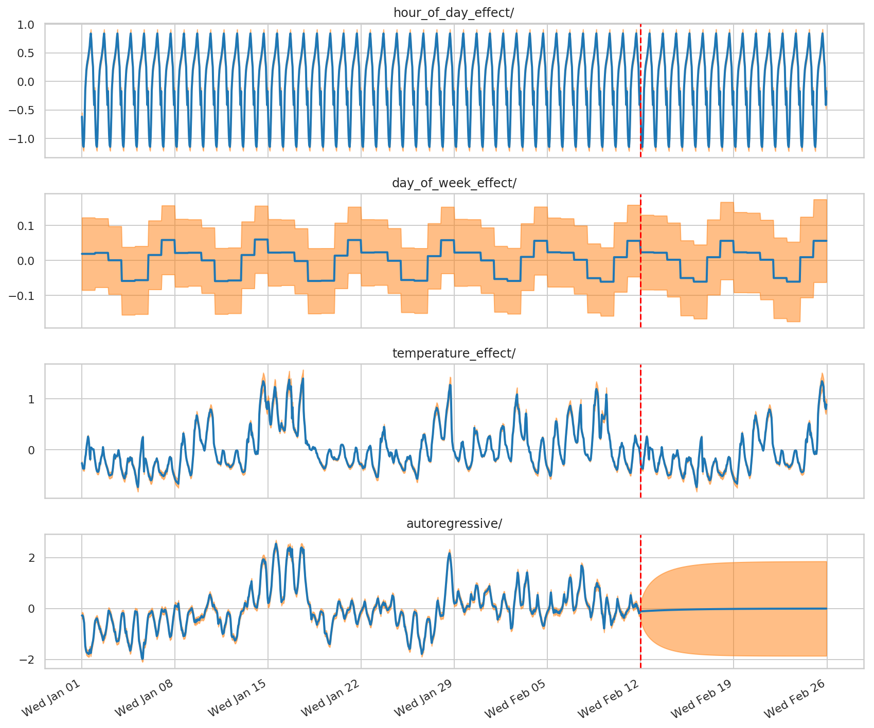
แบบจำลองของเรารวมฤดูกาลของชั่วโมงของวันและวันในสัปดาห์ กับแบบจำลองการถดถอยเชิงเส้นที่จำลองผลกระทบของอุณหภูมิ และกระบวนการถดถอยอัตโนมัติเพื่อจัดการกับเศษที่เหลือจากความแปรปรวนที่มีขอบเขต
def build_model(observed_time_series):
  hour_of_day_effect = sts.Seasonal(
      num_seasons=24,
      observed_time_series=observed_time_series,
      name='hour_of_day_effect')
  day_of_week_effect = sts.Seasonal(
      num_seasons=7, num_steps_per_season=24,
      observed_time_series=observed_time_series,
      name='day_of_week_effect')
  temperature_effect = sts.LinearRegression(
      design_matrix=tf.reshape(temperature - np.mean(temperature),
                               (-1, 1)), name='temperature_effect')
  autoregressive = sts.Autoregressive(
      order=1,
      observed_time_series=observed_time_series,
      name='autoregressive')
  model = sts.Sum([hour_of_day_effect,
                   day_of_week_effect,
                   temperature_effect,
                   autoregressive],
                   observed_time_series=observed_time_series)
  return model
ดังที่กล่าวข้างต้น เราจะปรับโมเดลด้วยการอนุมานแบบแปรผันและดึงตัวอย่างจากด้านหลัง
demand_model = build_model(demand_training_data)

# Build the variational surrogate posteriors `qs`.
variational_posteriors = tfp.sts.build_factored_surrogate_posterior(
    model=demand_model)
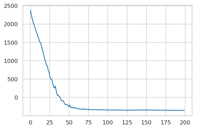
ลดการสูญเสียการแปรผันให้น้อยที่สุด
# Allow external control of optimization to reduce test runtimes.
num_variational_steps = 200 # @param { isTemplate: true}
num_variational_steps = int(num_variational_steps)

# Build and optimize the variational loss function.
elbo_loss_curve = tfp.vi.fit_surrogate_posterior(
    target_log_prob_fn=demand_model.joint_distribution(
        observed_time_series=demand_training_data).log_prob,
    surrogate_posterior=variational_posteriors,
    optimizer=tf.optimizers.Adam(learning_rate=0.1),
    num_steps=num_variational_steps,
    jit_compile=True)
plt.plot(elbo_loss_curve)
plt.show()

# Draw samples from the variational posterior.
q_samples_demand_ = variational_posteriors.sample(50)
print("Inferred parameters:")
for param in demand_model.parameters:
  print("{}: {} +- {}".format(param.name,
                              np.mean(q_samples_demand_[param.name], axis=0),
                              np.std(q_samples_demand_[param.name], axis=0)))
Inferred parameters:
observation_noise_scale: 0.010157477110624313 +- 0.0026443174574524164
hour_of_day_effect/_drift_scale: 0.0019522204529494047 +- 0.0011986979516223073
day_of_week_effect/_drift_scale: 0.013334915973246098 +- 0.01825258508324623
temperature_effect/_weights: [0.06648794] +- [0.00411669]
autoregressive/_coefficients: [0.9871232] +- [0.00413899]
autoregressive/_level_scale: 0.14199139177799225 +- 0.002658574376255274
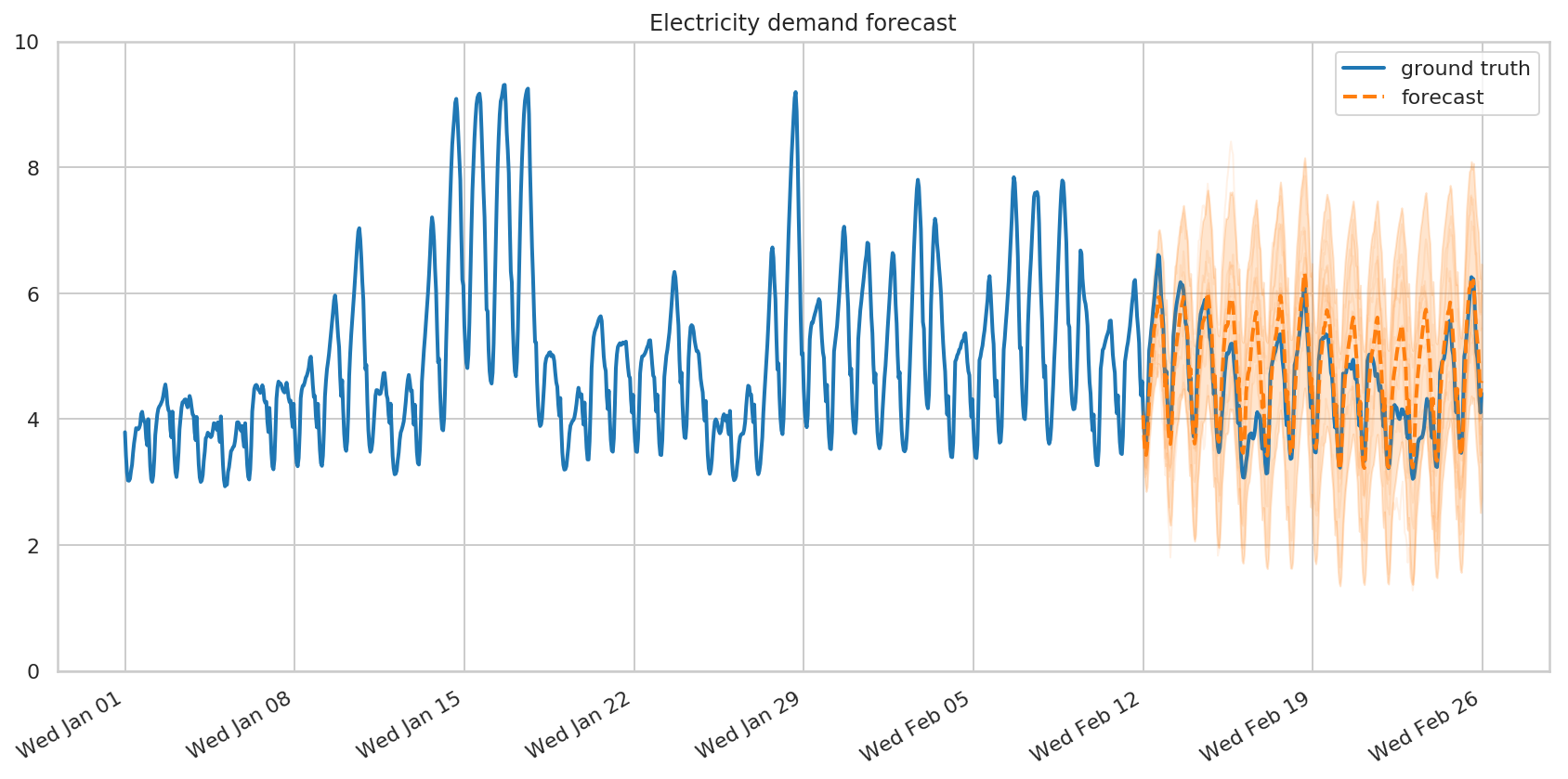
พยากรณ์และวิจารณ์
อีกครั้ง เราสร้างการคาดการณ์ง่ายๆ โดยการเรียก tfp.sts.forecast ด้วยโมเดล อนุกรมเวลา และพารามิเตอร์ตัวอย่างของเรา
demand_forecast_dist = tfp.sts.forecast(
    model=demand_model,
    observed_time_series=demand_training_data,
    parameter_samples=q_samples_demand_,
    num_steps_forecast=num_forecast_steps)
num_samples=10

(
    demand_forecast_mean,
    demand_forecast_scale,
    demand_forecast_samples
) = (
    demand_forecast_dist.mean().numpy()[..., 0],
    demand_forecast_dist.stddev().numpy()[..., 0],
    demand_forecast_dist.sample(num_samples).numpy()[..., 0]
    )
fig, ax = plot_forecast(demand_dates, demand,
                        demand_forecast_mean,
                        demand_forecast_scale,
                        demand_forecast_samples,
                        title="Electricity demand forecast",
                        x_locator=demand_loc, x_formatter=demand_fmt)
ax.set_ylim([0, 10])
fig.tight_layout()
ลองนึกภาพการสลายตัวของชุดข้อมูลที่สังเกตและคาดการณ์เป็นส่วนประกอบแต่ละส่วน:
# Get the distributions over component outputs from the posterior marginals on
# training data, and from the forecast model.
component_dists = sts.decompose_by_component(
    demand_model,
    observed_time_series=demand_training_data,
    parameter_samples=q_samples_demand_)

forecast_component_dists = sts.decompose_forecast_by_component(
    demand_model,
    forecast_dist=demand_forecast_dist,
    parameter_samples=q_samples_demand_)
demand_component_means_, demand_component_stddevs_ = (
    {k.name: c.mean() for k, c in component_dists.items()},
    {k.name: c.stddev() for k, c in component_dists.items()})

(
    demand_forecast_component_means_,
    demand_forecast_component_stddevs_
) = (
    {k.name: c.mean() for k, c in forecast_component_dists.items()},
    {k.name: c.stddev() for k, c in forecast_component_dists.items()}
    )
# Concatenate the training data with forecasts for plotting.
component_with_forecast_means_ = collections.OrderedDict()
component_with_forecast_stddevs_ = collections.OrderedDict()
for k in demand_component_means_.keys():
  component_with_forecast_means_[k] = np.concatenate([
      demand_component_means_[k],
      demand_forecast_component_means_[k]], axis=-1)
  component_with_forecast_stddevs_[k] = np.concatenate([
      demand_component_stddevs_[k],
      demand_forecast_component_stddevs_[k]], axis=-1)


fig, axes = plot_components(
  demand_dates,
  component_with_forecast_means_,
  component_with_forecast_stddevs_,
  x_locator=demand_loc, x_formatter=demand_fmt)
for ax in axes.values():
  ax.axvline(demand_dates[-num_forecast_steps], linestyle="--", color='red')
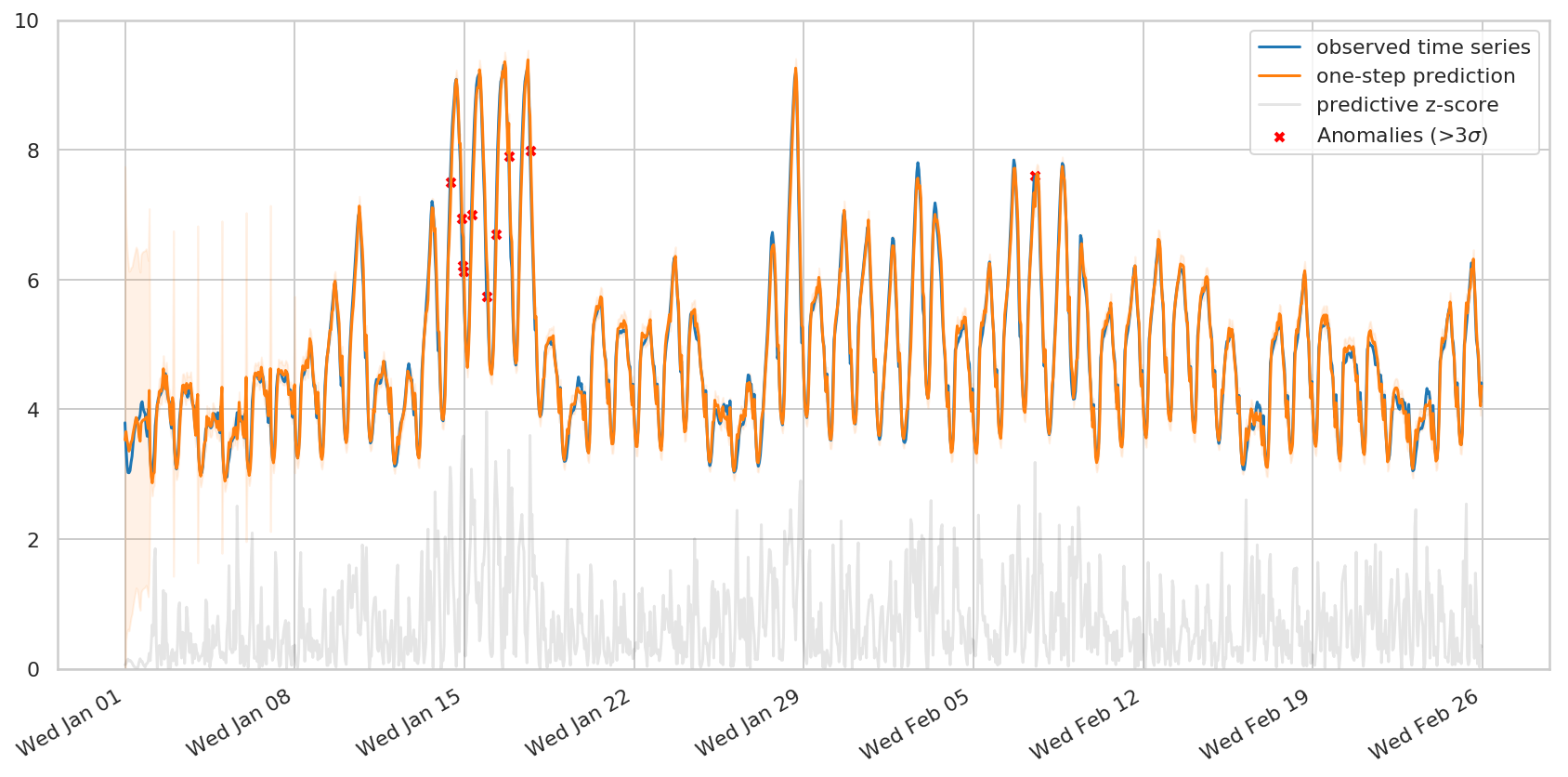
หากเราต้องการตรวจจับความผิดปกติในชุดข้อมูลที่สังเกตได้ เราอาจสนใจการแจกแจงแบบคาดการณ์ขั้นตอนเดียว นั่นคือ การคาดการณ์สำหรับแต่ละขั้นตอน โดยให้เฉพาะขั้นตอนจนถึงจุดนั้น tfp.sts.one_step_predictive คำนวณการแจกแจงแบบคาดการณ์ขั้นตอนเดียวทั้งหมดในครั้งเดียว:
demand_one_step_dist = sts.one_step_predictive(
    demand_model,
    observed_time_series=demand,
    parameter_samples=q_samples_demand_)

demand_one_step_mean, demand_one_step_scale = (
    demand_one_step_dist.mean().numpy(), demand_one_step_dist.stddev().numpy())
รูปแบบการตรวจจับความผิดปกติอย่างง่ายคือการแฟล็กขั้นตอนเวลาทั้งหมดที่การสังเกตมีค่ามากกว่าสาม stddevs จากค่าที่คาดการณ์ ซึ่งเป็นขั้นตอนที่ 'น่าประหลาดใจ' ที่สุดตามแบบจำลอง
fig, ax = plot_one_step_predictive(
    demand_dates, demand,
    demand_one_step_mean, demand_one_step_scale,
    x_locator=demand_loc, x_formatter=demand_fmt)
ax.set_ylim(0, 10)

# Use the one-step-ahead forecasts to detect anomalous timesteps.
zscores = np.abs((demand - demand_one_step_mean) /
                 demand_one_step_scale)
anomalies = zscores > 3.0
ax.scatter(demand_dates[anomalies],
           demand[anomalies],
           c="red", marker="x", s=20, linewidth=2, label=r"Anomalies (>3$\sigma$)")
ax.plot(demand_dates, zscores, color="black", alpha=0.1, label='predictive z-score')
ax.legend()
plt.show()