
| | |  ดูแหล่งที่มาบน GitHub ดูแหล่งที่มาบน GitHub |
ฉันเขียนสมุดบันทึกนี้เป็นกรณีศึกษาเพื่อเรียนรู้ความน่าจะเป็นของ TensorFlow ปัญหาที่ฉันเลือกแก้ไขคือการประมาณเมทริกซ์ความแปรปรวนร่วมสำหรับตัวอย่างของตัวแปรสุ่ม 2 มิติเฉลี่ย 0 เกาส์เซียน ปัญหามีคุณสมบัติที่ดีสองสามอย่าง:
- หากเราใช้ Wishart แบบผกผันก่อนสำหรับความแปรปรวนร่วม (แนวทางทั่วไป) ปัญหาจะมีวิธีการวิเคราะห์ ดังนั้นเราจึงสามารถตรวจสอบผลลัพธ์ของเราได้
- ปัญหาเกี่ยวข้องกับการสุ่มตัวอย่างพารามิเตอร์ที่มีข้อจำกัด ซึ่งเพิ่มความซับซ้อนที่น่าสนใจบางอย่าง
- วิธีแก้ปัญหาที่ตรงไปตรงมาที่สุดไม่ใช่วิธีที่เร็วที่สุด ดังนั้นจึงมีงานเพิ่มประสิทธิภาพบางอย่างที่ต้องทำ
ฉันตัดสินใจที่จะเขียนประสบการณ์ของฉันในขณะที่ฉันไป ฉันใช้เวลาสักครู่ในการพิจารณาจุดเล็กๆ น้อยๆ ของ TFP โน้ตบุ๊กนี้จึงเริ่มต้นได้ค่อนข้างง่าย และค่อยๆ ทำงานกับคุณลักษณะ TFP ที่ซับซ้อนมากขึ้นเรื่อยๆ ฉันพบปัญหามากมายระหว่างทาง และฉันพยายามรวบรวมทั้งกระบวนการที่ช่วยให้ฉันระบุได้ และวิธีแก้ไขปัญหาเฉพาะหน้าที่ฉันพบในที่สุด ฉันได้พยายามที่จะรวมถึงจำนวนมากของรายละเอียด (รวมถึงจำนวนมากของการทดสอบเพื่อให้แน่ใจว่าแต่ละขั้นตอนที่ถูกต้อง)
ทำไมต้องเรียนรู้ความน่าจะเป็นของ TensorFlow
ฉันพบว่า TensorFlow Probability น่าสนใจสำหรับโครงการของฉันด้วยเหตุผลบางประการ:
- ความน่าจะเป็นของ TensorFlow ช่วยให้คุณสร้างต้นแบบในการพัฒนาแบบจำลองที่ซับซ้อนแบบโต้ตอบได้ในโน้ตบุ๊ก คุณสามารถแบ่งรหัสของคุณออกเป็นชิ้นเล็ก ๆ ที่คุณสามารถทดสอบแบบโต้ตอบและด้วยการทดสอบหน่วย
- เมื่อคุณพร้อมที่จะขยายขนาดแล้ว คุณสามารถใช้ประโยชน์จากโครงสร้างพื้นฐานทั้งหมดที่เรามีเพื่อให้ TensorFlow ทำงานบนโปรเซสเซอร์ที่ปรับให้เหมาะสมหลายตัวบนหลายเครื่อง
- สุดท้ายนี้ ในขณะที่ฉันชอบสแตนมาก ฉันพบว่ามันค่อนข้างยากที่จะแก้ไขจุดบกพร่อง คุณต้องเขียนโค้ดการสร้างโมเดลทั้งหมดในภาษาแบบสแตนด์อโลนที่มีเครื่องมือน้อยมากที่จะช่วยให้คุณเจาะโค้ด ตรวจสอบสถานะระหว่างกลาง และอื่นๆ
ข้อเสียคือความน่าจะเป็นของ TensorFlow นั้นใหม่กว่า Stan และ PyMC3 มาก ดังนั้นเอกสารประกอบจึงอยู่ในระหว่างดำเนินการ และมีฟังก์ชันมากมายที่ยังไม่ได้สร้างขึ้น อย่างมีความสุข ฉันพบว่ารากฐานของ TFP นั้นแข็งแกร่ง และได้รับการออกแบบในลักษณะโมดูลาร์ที่ช่วยให้สามารถขยายฟังก์ชันการทำงานได้ค่อนข้างตรงไปตรงมา ในสมุดบันทึกนี้ นอกจากการแก้ปัญหากรณีศึกษาแล้ว ฉันจะแสดงวิธีต่างๆ ในการขยาย TFP
นี้เพื่อใคร
ฉันคิดว่าผู้อ่านจะมาที่สมุดบันทึกนี้โดยมีข้อกำหนดเบื้องต้นที่สำคัญบางประการ คุณควร:
- รู้พื้นฐานของการอนุมานแบบเบย์ (หากคุณไม่ได้เป็นหนังสือเล่มแรกที่ดีจริงๆเป็น สถิติทบทวน )
- มีความคุ้นเคยกับห้องสมุดสุ่มตัวอย่าง MCMC เช่นบาง แตน / PyMC3 / ข้อบกพร่อง
- มีความเข้าใจที่มั่นคงของ NumPy (หนึ่งบทนำที่ดีคือ งูใหญ่สำหรับการวิเคราะห์ข้อมูล )
- มีความคุ้นเคยผ่านน้อยกับ TensorFlow แต่ไม่จำเป็นต้องเชี่ยวชาญ ( เรียนรู้ TensorFlow เป็นสิ่งที่ดี แต่ TensorFlow อย่างรวดเร็ววิวัฒนาการหมายความว่าหนังสือส่วนใหญ่จะได้รับการบิตลงวันที่. สแตนฟอ CS20 แน่นอนนอกจากนี้ยังเป็นสิ่งที่ดี.)
ความพยายามครั้งแรก
นี่เป็นความพยายามครั้งแรกของฉันที่ปัญหา สปอยเลอร์: วิธีแก้ปัญหาของฉันใช้ไม่ได้ และจะต้องพยายามหลายครั้งเพื่อให้ทุกอย่างถูกต้อง! แม้ว่ากระบวนการจะใช้เวลาสักครู่ แต่ความพยายามด้านล่างแต่ละครั้งมีประโยชน์สำหรับการเรียนรู้ส่วนใหม่ของ TFP
หมายเหตุหนึ่ง: ปัจจุบัน TFP ไม่ได้ใช้การกระจาย Wishart แบบผกผัน (เราจะดูในตอนท้ายว่าจะหมุน Wishart ผกผันของเราเองได้อย่างไร) ดังนั้นฉันจะเปลี่ยนปัญหาเป็นการประมาณค่าเมทริกซ์ที่แม่นยำโดยใช้ Wishart ก่อน
import collections
import math
import os
import time

import numpy as np
import pandas as pd
import scipy
import scipy.stats
import matplotlib.pyplot as plt

import tensorflow.compat.v2 as tf
tf.enable_v2_behavior()
import tensorflow_probability as tfp
tfd = tfp.distributions
tfb = tfp.bijectors
ขั้นตอนที่ 1: รับการสังเกตด้วยกัน
ข้อมูลของฉันที่นี่เป็นข้อมูลสังเคราะห์ทั้งหมด ดังนั้นข้อมูลนี้จะดูเป็นระเบียบกว่าตัวอย่างในโลกแห่งความเป็นจริงเล็กน้อย อย่างไรก็ตาม ไม่มีเหตุผลใดที่คุณไม่สามารถสร้างข้อมูลสังเคราะห์ของคุณเองได้
เคล็ดลับ: เมื่อคุณได้ตัดสินใจเกี่ยวกับรูปแบบของรูปแบบของคุณคุณสามารถเลือกค่าพารามิเตอร์บางอย่างและใช้รูปแบบที่คุณเลือกในการสร้างข้อมูลสังเคราะห์บาง ในการตรวจสอบความสมบูรณ์ของการนำไปใช้ของคุณ คุณสามารถตรวจสอบได้ว่าค่าประมาณของคุณรวมค่าที่แท้จริงของพารามิเตอร์ที่คุณเลือกไว้ เพื่อให้การดีบัก / รอบการทดสอบของคุณเร็วขึ้น คุณอาจพิจารณารุ่นที่เรียบง่ายของโมเดลของคุณ (เช่น ใช้มิติข้อมูลน้อยลงหรือตัวอย่างน้อยลง)
เคล็ดลับ: มันเป็นเรื่องที่ง่ายที่สุดในการทำงานกับข้อสังเกตของคุณเป็นอาร์เรย์ NumPy สิ่งสำคัญประการหนึ่งที่ควรทราบคือโดยค่าเริ่มต้น NumPy จะใช้ของ float64 ในขณะที่ TensorFlow โดยค่าเริ่มต้นจะใช้ของ float32
โดยทั่วไป การดำเนินการของ TensorFlow ต้องการให้อาร์กิวเมนต์ทั้งหมดมีประเภทเดียวกัน และคุณต้องทำการแคสต์ข้อมูลอย่างชัดเจนเพื่อเปลี่ยนประเภท หากคุณใช้การสังเกต float64 คุณจะต้องเพิ่มการดำเนินการแคสต์จำนวนมาก ในทางกลับกัน NumPy จะดูแลการแคสต์โดยอัตโนมัติ จึงเป็นเรื่องง่ายที่จะแปลงข้อมูล Numpy ของคุณลงใน float32 กว่าก็คือการบังคับ TensorFlow กับการใช้ float64
เลือกค่าพารามิเตอร์บางค่า
# We're assuming 2-D data with a known true mean of (0, 0)
true_mean = np.zeros([2], dtype=np.float32)
# We'll make the 2 coordinates correlated
true_cor = np.array([[1.0, 0.9], [0.9, 1.0]], dtype=np.float32)
# And we'll give the 2 coordinates different variances
true_var = np.array([4.0, 1.0], dtype=np.float32)
# Combine the variances and correlations into a covariance matrix
true_cov = np.expand_dims(np.sqrt(true_var), axis=1).dot(
    np.expand_dims(np.sqrt(true_var), axis=1).T) * true_cor
# We'll be working with precision matrices, so we'll go ahead and compute the
# true precision matrix here
true_precision = np.linalg.inv(true_cov)
# Here's our resulting covariance matrix
print(true_cov)
# Verify that it's positive definite, since np.random.multivariate_normal
# complains about it not being positive definite for some reason.
# (Note that I'll be including a lot of sanity checking code in this notebook -
# it's a *huge* help for debugging)
print('eigenvalues: ', np.linalg.eigvals(true_cov))
[[4.  1.8]
 [1.8 1. ]]
eigenvalues:  [4.843075   0.15692513]
สร้างข้อสังเกตสังเคราะห์บางอย่าง
โปรดทราบว่า TensorFlow น่าจะใช้การประชุมว่ามิติเริ่มต้น (s) ของข้อมูลของคุณแทนดัชนีตัวอย่างและมิติสุดท้าย (s) ของข้อมูลของคุณหมายถึงมิติของกลุ่มตัวอย่างของคุณ
ที่นี่เราต้องการ 100 ตัวอย่างซึ่งแต่ละเป็นเวกเตอร์ของความยาว 2. เราจะสร้างอาร์เรย์ my_data มีรูปร่าง (100, 2) my_data[i, :] เป็น \(i\)ตัวอย่าง, th และมันเป็นเวกเตอร์ของความยาว 2
(อย่าลืมที่จะทำให้ my_data มีประเภท float32!)
# Set the seed so the results are reproducible.
np.random.seed(123)

# Now generate some observations of our random variable.
# (Note that I'm suppressing a bunch of spurious about the covariance matrix
# not being positive semidefinite via check_valid='ignore' because it really is
# positive definite!)
my_data = np.random.multivariate_normal(
    mean=true_mean, cov=true_cov, size=100,
    check_valid='ignore').astype(np.float32)
my_data.shape
(100, 2)
สติตรวจสอบข้อสังเกต
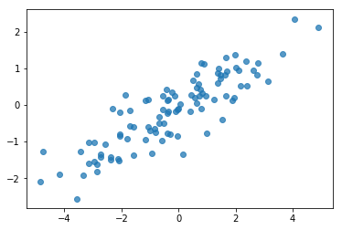
แหล่งที่มาของข้อบกพร่องที่อาจเกิดขึ้นได้ทำให้ข้อมูลสังเคราะห์ของคุณยุ่งเหยิง! มาทำการตรวจสอบง่ายๆ กัน
# Do a scatter plot of the observations to make sure they look like what we
# expect (higher variance on the x-axis, y values strongly correlated with x)
plt.scatter(my_data[:, 0], my_data[:, 1], alpha=0.75)
plt.show()
print('mean of observations:', np.mean(my_data, axis=0))
print('true mean:', true_mean)
mean of observations: [-0.24009615 -0.16638893]
true mean: [0. 0.]
print('covariance of observations:\n', np.cov(my_data, rowvar=False))
print('true covariance:\n', true_cov)
covariance of observations:
 [[3.95307734 1.68718486]
 [1.68718486 0.94910269]]
true covariance:
 [[4.  1.8]
 [1.8 1. ]]
โอเค ตัวอย่างของเราดูสมเหตุสมผล ขั้นตอนต่อไป.
ขั้นตอนที่ 2: ใช้ฟังก์ชันความน่าจะเป็นใน NumPy
สิ่งสำคัญที่เราจะต้องเขียนเพื่อทำการสุ่มตัวอย่าง MCMC ของเราในความน่าจะเป็น TF คือฟังก์ชันความน่าจะเป็นของบันทึก โดยทั่วไปแล้วการเขียน TF นั้นยากกว่า NumPy เล็กน้อย ดังนั้นฉันจึงพบว่าการนำไปใช้งานเบื้องต้นใน NumPy นั้นมีประโยชน์ ฉันจะแยกฟังก์ชั่นความน่าจะเป็น 2 ชิ้น, ฟังก์ชั่นข้อมูลความน่าจะเป็นที่สอดคล้องกับ \(P(data | parameters)\) และฟังก์ชั่นความน่าจะเป็นก่อนที่สอดคล้องกับ \(P(parameters)\)
โปรดทราบว่าฟังก์ชัน NumPy เหล่านี้ไม่จำเป็นต้องได้รับการปรับให้เหมาะสมที่สุด / แปลงเวกเตอร์เนื่องจากเป้าหมายคือการสร้างค่าบางอย่างสำหรับการทดสอบเท่านั้น ความถูกต้องคือการพิจารณาที่สำคัญ!
ขั้นแรกเราจะนำชิ้นส่วนความเป็นไปได้ในการบันทึกข้อมูล ที่ค่อนข้างตรงไปตรงมา สิ่งหนึ่งที่ต้องจำไว้คือเราจะทำงานกับเมทริกซ์ที่มีความแม่นยำ ดังนั้นเราจะสร้างพารามิเตอร์ตามนั้น
def log_lik_data_numpy(precision, data):
  # np.linalg.inv is a really inefficient way to get the covariance matrix, but
  # remember we don't care about speed here
  cov = np.linalg.inv(precision)
  rv = scipy.stats.multivariate_normal(true_mean, cov)
  return np.sum(rv.logpdf(data))

# test case: compute the log likelihood of the data given the true parameters
log_lik_data_numpy(true_precision, my_data)
-280.81822950593767
เรากำลังจะใช้ริชาร์ตก่อนสำหรับเมทริกซ์ที่มีความแม่นยำเนื่องจากมีวิธีการแก้ปัญหาการวิเคราะห์หลัง (ดู ตารางที่มีประโยชน์ของวิกิพีเดียไพรเออร์คอนจูเกต )
กระจายริชาร์ต มี 2 พารามิเตอร์:
- จำนวนองศาของเสรีภาพ (มีป้ายกำกับ \(\nu\) ในวิกิพีเดีย)
- เมทริกซ์ขนาด (มีป้ายกำกับ \(V\) ในวิกิพีเดีย)
ค่าเฉลี่ยสำหรับการกระจายริชาร์ตกับพารามิเตอร์ \(\nu, V\) เป็น \(E[W] = \nu V\)และความแปรปรวนเป็น \(\text{Var}(W_{ij}) = \nu(v_{ij}^2+v_{ii}v_{jj})\)
บางสัญชาตญาณที่มีประโยชน์: คุณสามารถสร้างตัวอย่างริชาร์ตโดยการสร้าง \(\nu\) อิสระดึง \(x_1 \ldots x_{\nu}\) จากตัวแปรสุ่มแบบหลายตัวแปรปกติที่มีค่าเฉลี่ย 0 และแปรปรวน \(V\) แล้วสร้างผลรวม \(W = \sum_{i=1}^{\nu} x_i x_i^T\)
หากคุณ rescale ตัวอย่างริชาร์ตโดยการหารพวกเขาโดย \(\nu\)คุณจะได้รับเมทริกซ์ความแปรปรวนตัวอย่างของ \(x_i\)ตัวอย่างแปรปรวนเมทริกซ์นี้ควรจะมีแนวโน้มไป \(V\) เป็น \(\nu\) เพิ่มขึ้น เมื่อ \(\nu\) มีขนาดเล็กมีจำนวนมากของการเปลี่ยนแปลงในเมทริกซ์ความแปรปรวนตัวอย่างขนาดเล็กเพื่อให้ค่าของ \(\nu\) สอดคล้องกับไพรเออร์ปรับตัวลดลงและค่านิยมที่มีขนาดใหญ่ของ \(\nu\) สอดคล้องกับไพรเออร์ที่แข็งแกร่ง โปรดทราบว่า \(\nu\) ต้องมีอย่างน้อยมีขนาดใหญ่เป็นมิติของพื้นที่ที่คุณกำลังสุ่มตัวอย่างหรือคุณจะสร้างเมทริกซ์เอกพจน์
เราจะใช้ \(\nu = 3\) เพื่อให้เรามีความอ่อนแอก่อนและเราจะใช้เวลา \(V = \frac{1}{\nu} I\) ซึ่งจะดึงประมาณการความแปรปรวนของเราที่มีต่อตัวตน (จำได้ว่าหมายถึงเป็น \(\nu V\))
PRIOR_DF = 3
PRIOR_SCALE = np.eye(2, dtype=np.float32) / PRIOR_DF

def log_lik_prior_numpy(precision):
  rv = scipy.stats.wishart(df=PRIOR_DF, scale=PRIOR_SCALE)
  return rv.logpdf(precision)

# test case: compute the prior for the true parameters
log_lik_prior_numpy(true_precision)
-9.103606346649766
มีการกระจายของริชาร์ตเป็นคอนจูเกตก่อนสำหรับการประเมินเมทริกซ์ที่มีความแม่นยำของหลายตัวแปรปกติที่มีค่าเฉลี่ยที่รู้จักกัน \(\mu\)
สมมติว่าพารามิเตอร์ริชาร์ตก่อนเป็น \(\nu, V\) และที่เรามี \(n\) สังเกตของเราหลายตัวแปรปกติ \(x_1, \ldots, x_n\)พารามิเตอร์หลังมี \(n + \nu, \left(V^{-1} + \sum_{i=1}^n (x_i-\mu)(x_i-\mu)^T \right)^{-1}\)
n = my_data.shape[0]
nu_prior = PRIOR_DF
v_prior = PRIOR_SCALE
nu_posterior = nu_prior + n
v_posterior = np.linalg.inv(np.linalg.inv(v_prior) + my_data.T.dot(my_data))
posterior_mean = nu_posterior * v_posterior
v_post_diag = np.expand_dims(np.diag(v_posterior), axis=1)
posterior_sd = np.sqrt(nu_posterior *
                       (v_posterior ** 2.0 + v_post_diag.dot(v_post_diag.T)))
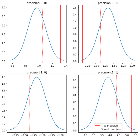
พล็อตเรื่องหลังและคุณค่าที่แท้จริงอย่างรวดเร็ว โปรดทราบว่าส่วนหลังจะอยู่ใกล้กับตัวอย่างด้านหลัง แต่จะหดตัวเล็กน้อยเพื่ออัตลักษณ์ โปรดทราบด้วยว่าค่าที่แท้จริงนั้นค่อนข้างห่างไกลจากโหมดของค่าหลัง - น่าจะเป็นเพราะค่าก่อนหน้านั้นไม่ตรงกับข้อมูลของเรามากนัก ในปัญหาที่แท้จริงที่เราต้องการจะทำอย่างไรดีกับสิ่งที่ต้องการปรับสัดส่วนผกผันริชาร์ตก่อนสำหรับความแปรปรวน (ดูตัวอย่างเช่นแอนดรู Gelman ของ ความเห็น เกี่ยวกับเรื่องนี้) แต่เราก็ไม่น่าจะมีหลังการวิเคราะห์ที่ดี
sample_precision = np.linalg.inv(np.cov(my_data, rowvar=False, bias=False))
fig, axes = plt.subplots(2, 2)
fig.set_size_inches(10, 10)
for i in range(2):
  for j in range(2):
    ax = axes[i, j]
    loc = posterior_mean[i, j]
    scale = posterior_sd[i, j]
    xmin = loc - 3.0 * scale
    xmax = loc + 3.0 * scale
    x = np.linspace(xmin, xmax, 1000)
    y = scipy.stats.norm.pdf(x, loc=loc, scale=scale)
    ax.plot(x, y)
    ax.axvline(true_precision[i, j], color='red', label='True precision')
    ax.axvline(sample_precision[i, j], color='red', linestyle=':', label='Sample precision')
    ax.set_title('precision[%d, %d]' % (i, j))
plt.legend()
plt.show()
ขั้นตอนที่ 3: ใช้ฟังก์ชันความน่าจะเป็นใน TensorFlow
สปอยเลอร์: ความพยายามครั้งแรกของเราไม่ได้ผล เราจะพูดถึงเหตุผลด้านล่าง
เคล็ดลับ: การใช้ TensorFlow โหมดความกระตือรือร้นที่เมื่อมีการพัฒนาฟังก์ชั่นโอกาสของ โหมดความกระตือรือร้นที่จะทำให้การทำงานของ TF มากขึ้นเช่น NumPy - รันทุกอย่างในทันทีเพื่อให้คุณสามารถแก้ปัญหาการโต้ตอบแทนที่จะต้องใช้ Session.run() ดูโน้ต ที่นี่
เบื้องต้น: คลาสการกระจาย
TFP มีคอลเล็กชันคลาสการแจกจ่ายที่เราจะใช้เพื่อสร้างความน่าจะเป็นของบันทึก สิ่งหนึ่งที่ควรทราบคือคลาสเหล่านี้ทำงานกับเทนเซอร์ของตัวอย่างมากกว่าแค่ตัวอย่างเดียว - ซึ่งช่วยให้สามารถเวกเตอร์และการเร่งความเร็วที่เกี่ยวข้องได้
การกระจายสามารถทำงานกับเทนเซอร์ของตัวอย่างได้ 2 วิธี ง่ายที่สุดที่จะแสดงให้เห็น 2 วิธีเหล่านี้ด้วยตัวอย่างที่เป็นรูปธรรมที่เกี่ยวข้องกับการแจกแจงด้วยพารามิเตอร์สเกลาร์เดียว ฉันจะใช้ Poisson กระจายซึ่งมี rate ค่าพารามิเตอร์
- ถ้าเราสร้าง Poisson มีมูลค่าเดียวสำหรับ
rateพารามิเตอร์การเรียกของsample()วิธีการส่งกลับค่าเดียว ค่านี้จะถูกเรียกว่าeventและในกรณีนี้เหตุการณ์ที่เกิดขึ้นเป็นสเกลาทั้งหมด - ถ้าเราสร้าง Poisson กับเมตริกซ์ของค่าสำหรับที่
rateพารามิเตอร์การเรียกของsample()วิธีการในขณะนี้จะส่งกลับค่าหลายหนึ่งสำหรับค่าในเมตริกซ์อัตราแต่ละ วัตถุที่ทำหน้าที่เป็นคอลเลกชันของ Poissons อิสระแต่ละคนมีอัตราของตัวเองและแต่ละค่าที่ส่งกลับโดยเรียกร้องให้sample()สอดคล้องกับหนึ่งใน Poissons เหล่านี้ คอลเลกชันของเหตุการณ์ที่เป็นอิสระ แต่ไม่กระจายเหมือนกันนี้เรียกว่าbatch -
sample()วิธีการใช้sample_shapeพารามิเตอร์ที่เริ่มต้นที่ tuple ที่ว่างเปล่า การส่งผ่านค่าที่ไม่ว่างเปล่าสำหรับsample_shapeผลในกลุ่มตัวอย่างกลับมาหลายชุด คอลเลกชันของแบตช์นี้เรียกว่าsample
กระจายของ log_prob() ข้อมูลวิธีการกินในลักษณะที่คล้ายคลึงกันว่า sample() สร้างมัน log_prob() ผลตอบแทนที่น่าจะเป็นตัวอย่างเช่นหลายกระบวนการที่เป็นอิสระจากเหตุการณ์ที่เกิดขึ้น
- ถ้าเรามีวัตถุ Poisson ของเราที่ถูกสร้างขึ้นด้วยสเกลา
rateแต่ละชุดเป็นสเกลาและถ้าเราผ่านในเมตริกซ์ของกลุ่มตัวอย่างที่เราจะได้รับการออกเมตริกซ์ที่มีขนาดเดียวกันของความน่าจะเข้าสู่ระบบ - ถ้าเรามีวัตถุ Poisson ของเราที่ถูกสร้างขึ้นด้วยเมตริกซ์ของรูปร่าง
Tของrateค่าแต่ละชุดเป็นเมตริกซ์ของรูปร่างTถ้าเราผ่านเทนเซอร์ของตัวอย่างรูปร่าง D, T, เราจะได้เทนเซอร์ของความน่าจะเป็นบันทึกของรูปร่าง D, T
ด้านล่างนี้คือตัวอย่างบางส่วนที่แสดงให้เห็นกรณีเหล่านี้ ดู สมุดบันทึกนี้ สำหรับการกวดวิชารายละเอียดเพิ่มเติมเกี่ยวกับเหตุการณ์ที่เกิดขึ้นสำหรับกระบวนการและรูปร่าง
# case 1: get log probabilities for a vector of iid draws from a single
# normal distribution
norm1 = tfd.Normal(loc=0., scale=1.)
probs1 = norm1.log_prob(tf.constant([1., 0.5, 0.]))

# case 2: get log probabilities for a vector of independent draws from
# multiple normal distributions with different parameters.  Note the vector
# values for loc and scale in the Normal constructor.
norm2 = tfd.Normal(loc=[0., 2., 4.], scale=[1., 1., 1.])
probs2 = norm2.log_prob(tf.constant([1., 0.5, 0.]))

print('iid draws from a single normal:', probs1.numpy())
print('draws from a batch of normals:', probs2.numpy())
iid draws from a single normal: [-1.4189385 -1.0439385 -0.9189385]
draws from a batch of normals: [-1.4189385 -2.0439386 -8.918939 ]
โอกาสในการบันทึกข้อมูล
ขั้นแรก เราจะใช้ฟังก์ชันความน่าจะเป็นในการบันทึกข้อมูล
VALIDATE_ARGS = True
ALLOW_NAN_STATS = False
ความแตกต่างที่สำคัญอย่างหนึ่งจากกรณี NumPy คือฟังก์ชันความน่าจะเป็นของ TensorFlow ของเราจะต้องจัดการกับเวกเตอร์ของเมทริกซ์ที่มีความแม่นยำมากกว่าแค่เมทริกซ์เดี่ยว เวกเตอร์ของพารามิเตอร์จะถูกใช้เมื่อเราสุ่มตัวอย่างจากหลายสาย
เราจะสร้างอ็อบเจ็กต์การแจกจ่ายที่ทำงานกับชุดของเมทริกซ์ที่มีความแม่นยำ (เช่น หนึ่งเมทริกซ์ต่อเชน)
เมื่อคำนวณความน่าจะเป็นบันทึกของข้อมูล เราจำเป็นต้องจำลองข้อมูลในลักษณะเดียวกับพารามิเตอร์ของเรา เพื่อให้มีสำเนาหนึ่งชุดต่อตัวแปรชุดงาน รูปร่างของข้อมูลที่ทำซ้ำของเราจะต้องเป็นดังนี้:
[sample shape, batch shape, event shape]
ในกรณีของเรา รูปร่างของเหตุการณ์คือ 2 (เนื่องจากเรากำลังทำงานกับเกาส์เซียนแบบ 2 มิติ) รูปร่างตัวอย่างคือ 100 เนื่องจากเรามีตัวอย่าง 100 ตัวอย่าง รูปร่างแบทช์จะเป็นจำนวนเมทริกซ์ความแม่นยำที่เรากำลังใช้อยู่ เป็นการสิ้นเปลืองที่จะทำซ้ำข้อมูลทุกครั้งที่เราเรียกใช้ฟังก์ชันความน่าจะเป็น ดังนั้นเราจะทำซ้ำข้อมูลล่วงหน้าและส่งต่อในเวอร์ชันที่จำลองแบบแล้ว
ทราบว่านี้คือการดำเนินการที่ไม่มีประสิทธิภาพ: MultivariateNormalFullCovariance เป็นญาติกับทางเลือกที่มีราคาแพงบางอย่างที่เราจะพูดถึงในส่วนของการเพิ่มประสิทธิภาพในตอนท้าย
def log_lik_data(precisions, replicated_data):
  n = tf.shape(precisions)[0]  # number of precision matrices
  # We're estimating a precision matrix; we have to invert to get log
  # probabilities.  Cholesky inversion should be relatively efficient,
  # but as we'll see later, it's even better if we can avoid doing the Cholesky
  # decomposition altogether.
  precisions_cholesky = tf.linalg.cholesky(precisions)
  covariances = tf.linalg.cholesky_solve(
      precisions_cholesky, tf.linalg.eye(2, batch_shape=[n]))
  rv_data = tfd.MultivariateNormalFullCovariance(
      loc=tf.zeros([n, 2]),
      covariance_matrix=covariances,
      validate_args=VALIDATE_ARGS,
      allow_nan_stats=ALLOW_NAN_STATS)

  return tf.reduce_sum(rv_data.log_prob(replicated_data), axis=0)
# For our test, we'll use a tensor of 2 precision matrices.
# We'll need to replicate our data for the likelihood function.
# Remember, TFP wants the data to be structured so that the sample dimensions
# are first (100 here), then the batch dimensions (2 here because we have 2
# precision matrices), then the event dimensions (2 because we have 2-D
# Gaussian data).  We'll need to add a middle dimension for the batch using
# expand_dims, and then we'll need to create 2 replicates in this new dimension
# using tile.
n = 2
replicated_data = np.tile(np.expand_dims(my_data, axis=1), reps=[1, 2, 1])
print(replicated_data.shape)
(100, 2, 2)
เคล็ดลับ: สิ่งหนึ่งที่ผมได้พบว่าเป็นประโยชน์อย่างมากคือการเขียนการตรวจสอบสุขภาพจิตดีเล็ก ๆ น้อย ๆ ของการทำงาน TensorFlow ของฉัน การทำให้เวกเตอร์ใน TF ยุ่งเหยิงนั้นง่ายมาก ดังนั้นการมีฟังก์ชัน NumPy ที่ง่ายกว่าจึงเป็นวิธีที่ดีในการตรวจสอบเอาต์พุต TF คิดว่าสิ่งเหล่านี้เป็นการทดสอบหน่วยเพียงเล็กน้อย
# check against the numpy implementation
precisions = np.stack([np.eye(2, dtype=np.float32), true_precision])
n = precisions.shape[0]
lik_tf = log_lik_data(precisions, replicated_data=replicated_data).numpy()

for i in range(n):
  print(i)
  print('numpy:', log_lik_data_numpy(precisions[i], my_data))
  print('tensorflow:', lik_tf[i])
0
numpy: -430.71218815801365
tensorflow: -430.71207
1
numpy: -280.81822950593767
tensorflow: -280.8182
โอกาสในการบันทึกก่อนหน้า
ก่อนหน้านั้นง่ายกว่าเนื่องจากเราไม่ต้องกังวลกับการจำลองข้อมูล
@tf.function(autograph=False)
def log_lik_prior(precisions):
  rv_precision = tfd.WishartTriL(
      df=PRIOR_DF,
      scale_tril=tf.linalg.cholesky(PRIOR_SCALE),
      validate_args=VALIDATE_ARGS,
      allow_nan_stats=ALLOW_NAN_STATS)
  return rv_precision.log_prob(precisions)
# check against the numpy implementation
precisions = np.stack([np.eye(2, dtype=np.float32), true_precision])
n = precisions.shape[0]
lik_tf = log_lik_prior(precisions).numpy()

for i in range(n):
  print(i)
  print('numpy:', log_lik_prior_numpy(precisions[i]))
  print('tensorflow:', lik_tf[i])
0
numpy: -2.2351873809649625
tensorflow: -2.2351875
1
numpy: -9.103606346649766
tensorflow: -9.103608
สร้างฟังก์ชั่นความเป็นไปได้ของบันทึกร่วม
ฟังก์ชันความเป็นไปได้ในการบันทึกข้อมูลด้านบนขึ้นอยู่กับการสังเกตของเรา แต่ตัวเก็บตัวอย่างจะไม่มี เราสามารถกำจัดการพึ่งพาโดยไม่ต้องใช้ตัวแปรส่วนกลางโดยใช้ [ปิด](https://en.wikipedia.org/wiki/Closure_(computer_programming) การปิดเกี่ยวข้องกับฟังก์ชันภายนอกที่สร้างสภาพแวดล้อมที่มีตัวแปรที่จำเป็น ฟังก์ชั่นภายใน
def get_log_lik(data, n_chains=1):
  # The data argument that is passed in will be available to the inner function
  # below so it doesn't have to be passed in as a parameter.
  replicated_data = np.tile(np.expand_dims(data, axis=1), reps=[1, n_chains, 1])

  @tf.function(autograph=False)
  def _log_lik(precision):
    return log_lik_data(precision, replicated_data) + log_lik_prior(precision)

  return _log_lik
ขั้นตอนที่ 4: ตัวอย่าง
โอเค ได้เวลาลองชิมแล้ว! เพื่อให้ง่ายขึ้น เราจะใช้ 1 เชน และเราจะใช้เมทริกซ์เอกลักษณ์เป็นจุดเริ่มต้น เราจะทำสิ่งต่าง ๆ อย่างระมัดระวังมากขึ้นในภายหลัง
อีกครั้ง วิธีนี้ใช้ไม่ได้ผล เราจะได้รับข้อยกเว้น
@tf.function(autograph=False)
def sample():
  tf.random.set_seed(123)
  init_precision = tf.expand_dims(tf.eye(2), axis=0)

  # Use expand_dims because we want to pass in a tensor of starting values
  log_lik_fn = get_log_lik(my_data, n_chains=1)

  # we'll just do a few steps here
  num_results = 10
  num_burnin_steps = 10
  states = tfp.mcmc.sample_chain(
     num_results=num_results,
     num_burnin_steps=num_burnin_steps,
     current_state=[
         init_precision,
     ],
     kernel=tfp.mcmc.HamiltonianMonteCarlo(
         target_log_prob_fn=log_lik_fn,
         step_size=0.1,
         num_leapfrog_steps=3),
     trace_fn=None,
     seed=123)
  return states

try:
  states = sample()
except Exception as e:
  # shorten the giant stack trace
  lines = str(e).split('\n')
  print('\n'.join(lines[:5]+['...']+lines[-3:]))
Cholesky decomposition was not successful. The input might not be valid.
     [[{ {node mcmc_sample_chain/trace_scan/while/body/_79/smart_for_loop/while/body/_371/mh_one_step/hmc_kernel_one_step/leapfrog_integrate/while/body/_537/leapfrog_integrate_one_step/maybe_call_fn_and_grads/value_and_gradients/StatefulPartitionedCall/Cholesky} }]] [Op:__inference_sample_2849]

Function call stack:
sample
...
Function call stack:
sample
การระบุปัญหา
InvalidArgumentError (see above for traceback): Cholesky decomposition was not successful. The input might not be valid. นั่นไม่เป็นประโยชน์อย่างยิ่ง ลองดูว่าเราสามารถหาข้อมูลเพิ่มเติมเกี่ยวกับสิ่งที่เกิดขึ้นได้หรือไม่
- เราจะพิมพ์พารามิเตอร์สำหรับแต่ละขั้นตอนเพื่อให้เห็นค่าของสิ่งที่ล้มเหลว
- เราจะเพิ่มการยืนยันเพื่อป้องกันปัญหาเฉพาะ
การยืนยันเป็นเรื่องยากเพราะเป็นการดำเนินการของ TensorFlow และเราต้องดูแลว่าการดำเนินการดังกล่าวจะได้รับการดำเนินการและไม่ได้รับการปรับให้เหมาะสมจากกราฟ มันคุ้มค่าที่อ่าน ภาพรวมนี้ ของ TensorFlow แก้จุดบกพร่องถ้าคุณไม่คุ้นเคยกับยืนยัน TF คุณสามารถบังคับให้ชัดเจนยืนยันที่จะดำเนินการโดยใช้ tf.control_dependencies (ดูความคิดเห็นในรหัสด้านล่าง)
TensorFlow พื้นเมือง Print ฟังก์ชั่นที่มีพฤติกรรมเช่นเดียวกับยืนยัน - มันดำเนินการและคุณจะต้องดูแลเพื่อให้แน่ใจว่าจะรัน Print ที่ทำให้เกิดอาการปวดหัวเพิ่มเติมเมื่อเรากำลังทำงานในสมุดบันทึก: ผลลัพธ์ที่ได้จะถูกส่งไป stderr และ stderr จะไม่ปรากฏในเซลล์ เราจะใช้เคล็ดลับที่นี่: แทนการใช้ tf.Print เราจะสร้างการดำเนินการพิมพ์ TensorFlow ของเราเองผ่าน tf.pyfunc เช่นเดียวกับการยืนยัน เราต้องตรวจสอบให้แน่ใจว่าวิธีการของเราดำเนินการ
def get_log_lik_verbose(data, n_chains=1):
  # The data argument that is passed in will be available to the inner function
  # below so it doesn't have to be passed in as a parameter.
  replicated_data = np.tile(np.expand_dims(data, axis=1), reps=[1, n_chains, 1])

  def _log_lik(precisions):
    # An internal method we'll make into a TensorFlow operation via tf.py_func
    def _print_precisions(precisions):
      print('precisions:\n', precisions)
      return False  # operations must return something!
    # Turn our method into a TensorFlow operation
    print_op = tf.compat.v1.py_func(_print_precisions, [precisions], tf.bool)

    # Assertions are also operations, and some care needs to be taken to ensure
    # that they're executed
    assert_op = tf.assert_equal(
        precisions, tf.linalg.matrix_transpose(precisions),
        message='not symmetrical', summarize=4, name='symmetry_check')

    # The control_dependencies statement forces its arguments to be executed
    # before subsequent operations
    with tf.control_dependencies([print_op, assert_op]):
      return (log_lik_data(precisions, replicated_data) +
              log_lik_prior(precisions))

  return _log_lik
@tf.function(autograph=False)
def sample():
  tf.random.set_seed(123)
  init_precision = tf.eye(2)[tf.newaxis, ...]
  log_lik_fn = get_log_lik_verbose(my_data)
  # we'll just do a few steps here
  num_results = 10
  num_burnin_steps = 10
  states = tfp.mcmc.sample_chain(
      num_results=num_results,
      num_burnin_steps=num_burnin_steps,
      current_state=[
          init_precision,
      ],
      kernel=tfp.mcmc.HamiltonianMonteCarlo(
          target_log_prob_fn=log_lik_fn,
          step_size=0.1,
          num_leapfrog_steps=3),
      trace_fn=None,
      seed=123)

try:
  states = sample()
except Exception as e:
  # shorten the giant stack trace
  lines = str(e).split('\n')
  print('\n'.join(lines[:5]+['...']+lines[-3:]))
precisions:
 [[[1. 0.]
  [0. 1.]]]
precisions:
 [[[1. 0.]
  [0. 1.]]]
precisions:
 [[[ 0.24315196 -0.2761638 ]
  [-0.33882257  0.8622    ]]]
 assertion failed: [not symmetrical] [Condition x == y did not hold element-wise:] [x (leapfrog_integrate_one_step/add:0) = ] [[[0.243151963 -0.276163787][-0.338822573 0.8622]]] [y (leapfrog_integrate_one_step/maybe_call_fn_and_grads/value_and_gradients/matrix_transpose/transpose:0) = ] [[[0.243151963 -0.338822573][-0.276163787 0.8622]]]
     [[{ {node mcmc_sample_chain/trace_scan/while/body/_96/smart_for_loop/while/body/_381/mh_one_step/hmc_kernel_one_step/leapfrog_integrate/while/body/_503/leapfrog_integrate_one_step/maybe_call_fn_and_grads/value_and_gradients/symmetry_check_1/Assert/AssertGuard/else/_577/Assert} }]] [Op:__inference_sample_4837]

Function call stack:
sample
...
Function call stack:
sample
ทำไมถึงล้มเหลว
ค่าพารามิเตอร์ใหม่ค่าแรกที่สุ่มตัวอย่างคือเมทริกซ์อสมมาตร นั่นทำให้การสลายตัวของ Cholesky ล้มเหลว เนื่องจากมีการกำหนดไว้สำหรับเมทริกซ์สมมาตร (และแน่นอนบวก) เท่านั้น
ปัญหาที่นี่คือพารามิเตอร์ที่เราสนใจคือเมทริกซ์ที่มีความแม่นยำ และเมทริกซ์ความแม่นยำจะต้องเป็นจริง สมมาตร และแน่นอนเป็นบวก ตัวอย่างไม่รู้อะไรเกี่ยวกับข้อจำกัดนี้ (ยกเว้นอาจจะผ่านการไล่ระดับสี) ดังนั้นจึงเป็นไปได้อย่างยิ่งที่ตัวอย่างจะเสนอค่าที่ไม่ถูกต้อง ซึ่งนำไปสู่ข้อยกเว้น โดยเฉพาะอย่างยิ่งถ้าขนาดขั้นตอนมีขนาดใหญ่
ด้วยตัวเก็บตัวอย่าง Hamiltonian Monte Carlo เราอาจสามารถแก้ไขปัญหาได้โดยใช้ขนาดขั้นตอนที่เล็กมาก เนื่องจากการไล่ระดับสีควรเก็บพารามิเตอร์ไว้ห่างจากบริเวณที่ไม่ถูกต้อง แต่ขนาดขั้นตอนขนาดเล็กหมายถึงการบรรจบกันที่ช้า ด้วยเครื่องเก็บตัวอย่าง Metropolis-Hastings ซึ่งไม่รู้อะไรเลยเกี่ยวกับการไล่ระดับสี เราถึงวาระแล้ว
เวอร์ชัน 2: การปรับพารามิเตอร์ใหม่เป็นพารามิเตอร์ที่ไม่มีข้อจำกัด
มีวิธีแก้ไขปัญหาข้างต้นอย่างตรงไปตรงมา: เราสามารถกำหนดพารามิเตอร์แบบจำลองของเราใหม่เพื่อให้พารามิเตอร์ใหม่ไม่มีข้อจำกัดเหล่านี้อีกต่อไป TFP มีชุดเครื่องมือที่มีประโยชน์ - bijectors - สำหรับการทำเช่นนั้น
การปรับพารามิเตอร์ใหม่ด้วย bijectors
เมทริกซ์ความแม่นยำของเราต้องเป็นจริงและสมมาตร เราต้องการพารามิเตอร์ทางเลือกที่ไม่มีข้อจำกัดเหล่านี้ จุดเริ่มต้นคือการแยกตัวประกอบของ Cholesky ของเมทริกซ์ความแม่นยำ ปัจจัย Cholesky ยังคงมีข้อจำกัด - พวกมันเป็นรูปสามเหลี่ยมล่าง และองค์ประกอบในแนวทแยงต้องเป็นค่าบวก อย่างไรก็ตาม หากเรานำบันทึกของเส้นทแยงมุมของปัจจัย Cholesky บันทึกจะไม่ถูกจำกัดให้เป็นค่าบวกอีกต่อไป จากนั้นหากเราแผ่ส่วนสามเหลี่ยมล่างให้เป็นเวกเตอร์ 1-D เราจะไม่มีข้อจำกัดรูปสามเหลี่ยมที่ต่ำกว่าอีกต่อไป . ผลลัพธ์ในกรณีของเราจะมีความยาว 3 เวกเตอร์โดยไม่มีข้อจำกัด
(ใน คู่มือแตน มีบทที่ดีเกี่ยวกับการใช้การเปลี่ยนแปลงที่จะลบประเภทต่างๆของข้อ จำกัด ในพารามิเตอร์.)
การปรับพารามิเตอร์ใหม่นี้มีผลเพียงเล็กน้อยต่อฟังก์ชันความเป็นไปได้ในการบันทึกข้อมูลของเรา - เราแค่ต้องกลับการแปลงของเรา เพื่อเราจะได้เมทริกซ์ที่มีความแม่นยำกลับคืนมา - แต่ผลกระทบที่เกิดก่อนหน้านั้นซับซ้อนกว่า เราได้ระบุว่าความน่าจะเป็นของเมทริกซ์ความแม่นยำที่กำหนดนั้นมาจากการแจกแจง Wishart ความน่าจะเป็นของเมทริกซ์ที่แปลงแล้วของเราเป็นเท่าไหร่?
จำได้ว่าถ้าเราใช้ฟังก์ชั่นต่อเนื่อง \(g\) ไป 1-D ตัวแปรสุ่ม \(X\), \(Y = g(X)\)ความหนาแน่นสำหรับ \(Y\) จะได้รับจาก
\[ f_Y(y) = | \frac{d}{dy}(g^{-1}(y)) | f_X(g^{-1}(y)) \]
อนุพันธ์ของ \(g^{-1}\) ระยะบัญชีสำหรับวิธีการที่ \(g\) เปลี่ยนแปลงปริมาณท้องถิ่น สำหรับสูงตัวแปรสุ่มมิติปัจจัยการแก้ไขเป็นค่าที่แน่นอนของปัจจัยของจาโคเบียนของ \(g^{-1}\) (ดู ที่นี่ )
เราจะต้องเพิ่มจาโคเบียนของการแปลงผกผันลงในฟังก์ชันความเป็นไปได้ของบันทึกก่อนหน้า อย่างมีความสุขของ TFP Bijector ระดับสามารถดูแลนี้สำหรับเรา
Bijector ระดับจะใช้เพื่อแสดงกลับด้านฟังก์ชั่นเรียบที่ใช้สำหรับการเปลี่ยนตัวแปรในฟังก์ชั่นความหนาแน่นของความน่าจะเป็น Bijectors ทุกคนมี forward() วิธีการที่จะดำเนินการเปลี่ยนการ inverse() วิธีการที่ตีความมันและ forward_log_det_jacobian() และ inverse_log_det_jacobian() วิธีการที่ให้แก้ไขจาโคเบียนเราต้องเมื่อเรา reparaterize ไฟล์ PDF
TFP ให้เก็บของ bijectors ที่มีประโยชน์ที่เราสามารถรวมผ่านองค์ประกอบผ่านมา Chain ผู้ประกอบการในรูปแบบการแปลงค่อนข้างซับซ้อน ในกรณีของเรา เราจะเขียน bijectors 3 ตัวต่อไปนี้ (การดำเนินการใน chain จะดำเนินการจากขวาไปซ้าย):
- ขั้นตอนแรกของการแปลงของเราคือทำการแยกตัวประกอบ Cholesky บนเมทริกซ์ที่มีความแม่นยำ ไม่มีคลาส Bijector สำหรับสิ่งนั้น แต่
CholeskyOuterProductbijector ต้องใช้ผลิตภัณฑ์จาก 2 ปัจจัย Cholesky เราสามารถใช้ผกผันของการดำเนินงานที่ใช้Invertผู้ประกอบการ - ขั้นตอนต่อไปคือการบันทึกองค์ประกอบในแนวทแยงของปัจจัย Cholesky เราบรรลุนี้ผ่านทาง
TransformDiagonalbijector และผกผันของExpbijector - ในที่สุดเราแผ่ส่วนสามเหลี่ยมล่างของเมทริกซ์เวกเตอร์โดยใช้ผกผันของ
FillTriangularbijector
# Our transform has 3 stages that we chain together via composition:
precision_to_unconstrained = tfb.Chain([
    # step 3: flatten the lower triangular portion of the matrix
    tfb.Invert(tfb.FillTriangular(validate_args=VALIDATE_ARGS)),
    # step 2: take the log of the diagonals
    tfb.TransformDiagonal(tfb.Invert(tfb.Exp(validate_args=VALIDATE_ARGS))),
    # step 1: decompose the precision matrix into its Cholesky factors
    tfb.Invert(tfb.CholeskyOuterProduct(validate_args=VALIDATE_ARGS)),
])
# sanity checks
m = tf.constant([[1., 2.], [2., 8.]])
m_fwd = precision_to_unconstrained.forward(m)
m_inv = precision_to_unconstrained.inverse(m_fwd)

# bijectors handle tensors of values, too!
m2 = tf.stack([m, tf.eye(2)])
m2_fwd = precision_to_unconstrained.forward(m2)
m2_inv = precision_to_unconstrained.inverse(m2_fwd)

print('single input:')
print('m:\n', m.numpy())
print('precision_to_unconstrained(m):\n', m_fwd.numpy())
print('inverse(precision_to_unconstrained(m)):\n', m_inv.numpy())
print()

print('tensor of inputs:')
print('m2:\n', m2.numpy())
print('precision_to_unconstrained(m2):\n', m2_fwd.numpy())
print('inverse(precision_to_unconstrained(m2)):\n', m2_inv.numpy())
single input:
m:
 [[1. 2.]
 [2. 8.]]
precision_to_unconstrained(m):
 [0.6931472 2.        0.       ]
inverse(precision_to_unconstrained(m)):
 [[1. 2.]
 [2. 8.]]

tensor of inputs:
m2:
 [[[1. 2.]
  [2. 8.]]

 [[1. 0.]
  [0. 1.]]]
precision_to_unconstrained(m2):
 [[0.6931472 2.        0.       ]
 [0.        0.        0.       ]]
inverse(precision_to_unconstrained(m2)):
 [[[1. 2.]
  [2. 8.]]

 [[1. 0.]
  [0. 1.]]]
TransformedDistribution ชั้นโดยอัตโนมัติกระบวนการของการใช้ bijector เพื่อกระจายและทำให้การแก้ไขจาโคเบียนที่จำเป็นในการ log_prob() ก่อนหน้าใหม่ของเรากลายเป็น:
def log_lik_prior_transformed(transformed_precisions):
  rv_precision = tfd.TransformedDistribution(
      tfd.WishartTriL(
          df=PRIOR_DF,
          scale_tril=tf.linalg.cholesky(PRIOR_SCALE),
          validate_args=VALIDATE_ARGS,
          allow_nan_stats=ALLOW_NAN_STATS),
      bijector=precision_to_unconstrained,
      validate_args=VALIDATE_ARGS)
  return rv_precision.log_prob(transformed_precisions)
# Check against the numpy implementation.  Note that when comparing, we need
# to add in the Jacobian correction.
precisions = np.stack([np.eye(2, dtype=np.float32), true_precision])
transformed_precisions = precision_to_unconstrained.forward(precisions)
lik_tf = log_lik_prior_transformed(transformed_precisions).numpy()
corrections = precision_to_unconstrained.inverse_log_det_jacobian(
    transformed_precisions, event_ndims=1).numpy()
n = precisions.shape[0]

for i in range(n):
  print(i)
  print('numpy:', log_lik_prior_numpy(precisions[i]) + corrections[i])
  print('tensorflow:', lik_tf[i])
0
numpy: -0.8488930160357633
tensorflow: -0.84889317
1
numpy: -7.305657151741624
tensorflow: -7.305659
เราเพียงแค่ต้องกลับการแปลงสำหรับโอกาสในการบันทึกข้อมูลของเรา:
precision = precision_to_unconstrained.inverse(transformed_precision)
เนื่องจากเราต้องการการแยกตัวประกอบของ Cholesky ของเมทริกซ์ความแม่นยำ การทำอินเวอร์สเพียงบางส่วนที่นี่จึงจะมีประสิทธิภาพมากกว่า อย่างไรก็ตาม เราจะปล่อยให้การปรับให้เหมาะสมในภายหลัง และจะปล่อยให้ส่วนผกผันบางส่วนเป็นแบบฝึกหัดสำหรับผู้อ่าน
def log_lik_data_transformed(transformed_precisions, replicated_data):
  # We recover the precision matrix by inverting our bijector.  This is
  # inefficient since we really want the Cholesky decomposition of the
  # precision matrix, and the bijector has that in hand during the inversion,
  # but we'll worry about efficiency later.
  n = tf.shape(transformed_precisions)[0]
  precisions = precision_to_unconstrained.inverse(transformed_precisions)
  precisions_cholesky = tf.linalg.cholesky(precisions)
  covariances = tf.linalg.cholesky_solve(
      precisions_cholesky, tf.linalg.eye(2, batch_shape=[n]))
  rv_data = tfd.MultivariateNormalFullCovariance(
      loc=tf.zeros([n, 2]),
      covariance_matrix=covariances,
      validate_args=VALIDATE_ARGS,
      allow_nan_stats=ALLOW_NAN_STATS)

  return tf.reduce_sum(rv_data.log_prob(replicated_data), axis=0)
# sanity check
precisions = np.stack([np.eye(2, dtype=np.float32), true_precision])
transformed_precisions = precision_to_unconstrained.forward(precisions)
lik_tf = log_lik_data_transformed(
    transformed_precisions, replicated_data).numpy()

for i in range(precisions.shape[0]):
  print(i)
  print('numpy:', log_lik_data_numpy(precisions[i], my_data))
  print('tensorflow:', lik_tf[i])
0
numpy: -430.71218815801365
tensorflow: -430.71207
1
numpy: -280.81822950593767
tensorflow: -280.8182
อีกครั้งเราห่อฟังก์ชันใหม่ของเราในการปิด
def get_log_lik_transformed(data, n_chains=1):
  # The data argument that is passed in will be available to the inner function
  # below so it doesn't have to be passed in as a parameter.
  replicated_data = np.tile(np.expand_dims(data, axis=1), reps=[1, n_chains, 1])

  @tf.function(autograph=False)
  def _log_lik_transformed(transformed_precisions):
    return (log_lik_data_transformed(transformed_precisions, replicated_data) +
            log_lik_prior_transformed(transformed_precisions))

  return _log_lik_transformed
# make sure everything runs
log_lik_fn = get_log_lik_transformed(my_data)
m = tf.eye(2)[tf.newaxis, ...]
lik = log_lik_fn(precision_to_unconstrained.forward(m)).numpy()
print(lik)
[-431.5611]
สุ่มตัวอย่าง
ตอนนี้เราไม่ต้องกังวลว่าตัวอย่างของเราจะระเบิดเนื่องจากค่าพารามิเตอร์ที่ไม่ถูกต้อง มาสร้างตัวอย่างจริงกัน
ตัวอย่างทำงานกับพารามิเตอร์ของเราในเวอร์ชันที่ไม่มีข้อจำกัด ดังนั้นเราจึงจำเป็นต้องแปลงค่าเริ่มต้นเป็นเวอร์ชันที่ไม่มีข้อจำกัด ตัวอย่างที่เราสร้างทั้งหมดจะอยู่ในรูปแบบที่ไม่มีข้อจำกัด ดังนั้นเราจำเป็นต้องแปลงกลับคืน Bijectors เป็น vectorized ดังนั้นจึงทำได้ง่าย
# We'll choose a proper random initial value this time
np.random.seed(123)
initial_value_cholesky = np.array(
    [[0.5 + np.random.uniform(), 0.0],
     [-0.5 + np.random.uniform(), 0.5 + np.random.uniform()]],
    dtype=np.float32)
initial_value =  initial_value_cholesky.dot(
  initial_value_cholesky.T)[np.newaxis, ...]

# The sampler works with unconstrained values, so we'll transform our initial
# value
initial_value_transformed = precision_to_unconstrained.forward(
  initial_value).numpy()
# Sample!
@tf.function(autograph=False)
def sample():
  tf.random.set_seed(123)
  log_lik_fn = get_log_lik_transformed(my_data, n_chains=1)

  num_results = 1000
  num_burnin_steps = 1000

  states, is_accepted = tfp.mcmc.sample_chain(
      num_results=num_results,
      num_burnin_steps=num_burnin_steps,
      current_state=[
          initial_value_transformed,
      ],
      kernel=tfp.mcmc.HamiltonianMonteCarlo(
          target_log_prob_fn=log_lik_fn,
          step_size=0.1,
          num_leapfrog_steps=3),
      trace_fn=lambda _, pkr: pkr.is_accepted,
      seed=123)
  # transform samples back to their constrained form
  precision_samples = [precision_to_unconstrained.inverse(s) for s in states]
  return states, precision_samples, is_accepted

states, precision_samples, is_accepted = sample()
มาเปรียบเทียบค่าเฉลี่ยของผลลัพธ์จากตัวอย่างของเรากับค่าเฉลี่ยส่วนหลังของการวิเคราะห์กัน!
print('True posterior mean:\n', posterior_mean)
print('Sample mean:\n', np.mean(np.reshape(precision_samples, [-1, 2, 2]), axis=0))
True posterior mean:
 [[ 0.9641779 -1.6534661]
 [-1.6534661  3.8683164]]
Sample mean:
 [[ 1.4315274  -0.25587553]
 [-0.25587553  0.5740424 ]]
เรามาไกลแล้ว! ลองหาสาเหตุ ก่อนอื่นมาดูตัวอย่างของเรากัน
np.reshape(precision_samples, [-1, 2, 2])
array([[[ 1.4315385, -0.2558777],
        [-0.2558777,  0.5740494]],

       [[ 1.4315385, -0.2558777],
        [-0.2558777,  0.5740494]],

       [[ 1.4315385, -0.2558777],
        [-0.2558777,  0.5740494]],

       ...,

       [[ 1.4315385, -0.2558777],
        [-0.2558777,  0.5740494]],

       [[ 1.4315385, -0.2558777],
        [-0.2558777,  0.5740494]],

       [[ 1.4315385, -0.2558777],
        [-0.2558777,  0.5740494]]], dtype=float32)
เอ่อ ดูเหมือนว่าพวกเขาทั้งหมดมีค่าเท่ากัน ลองหาสาเหตุ
kernel_results_ ตัวแปรเป็น tuple ชื่อที่ให้ข้อมูลเกี่ยวกับตัวอย่างในแต่ละรัฐ is_accepted ฟิลด์เป็นกุญแจสำคัญที่นี่
# Look at the acceptance for the last 100 samples
print(np.squeeze(is_accepted)[-100:])
print('Fraction of samples accepted:', np.mean(np.squeeze(is_accepted)))
[False False False False False False False False False False False False
 False False False False False False False False False False False False
 False False False False False False False False False False False False
 False False False False False False False False False False False False
 False False False False False False False False False False False False
 False False False False False False False False False False False False
 False False False False False False False False False False False False
 False False False False False False False False False False False False
 False False False False]
Fraction of samples accepted: 0.0
ตัวอย่างทั้งหมดของเราถูกปฏิเสธ! น่าจะเป็นขนาดก้าวของเราใหญ่เกินไป ผมเลือก stepsize=0.1 หมดจดโดยพลการ
เวอร์ชัน 3: การสุ่มตัวอย่างด้วยขนาดขั้นตอนที่ปรับเปลี่ยนได้
เนื่องจากการสุ่มตัวอย่างด้วยการเลือกขนาดขั้นตอนโดยพลการของฉันล้มเหลว เรามีวาระสองสามรายการ:
- ใช้ขนาดขั้นตอนที่ปรับเปลี่ยนได้และ
- ทำการตรวจสอบการบรรจบกัน
มีบางโค้ดตัวอย่างที่ดีในการเป็น tensorflow_probability/python/mcmc/hmc.py สำหรับการดำเนินการขั้นตอนการปรับตัวขนาด ฉันได้ดัดแปลงมันด้านล่าง
โปรดทราบว่ามีแยก sess.run() คำสั่งสำหรับแต่ละขั้นตอน สิ่งนี้มีประโยชน์จริง ๆ สำหรับการดีบัก เนื่องจากช่วยให้เราเพิ่มการวินิจฉัยทีละขั้นตอนได้อย่างง่ายดายหากจำเป็น ตัวอย่างเช่น เราสามารถแสดงความคืบหน้าที่เพิ่มขึ้น เวลาแต่ละขั้นตอน เป็นต้น
เคล็ดลับ: วิธีการหนึ่งที่เห็นได้ชัดว่าเป็นธรรมดาที่จะเลอะสุ่มตัวอย่างของคุณคือการมีการเจริญเติบโตกราฟของคุณในวง (เหตุผลในการสรุปกราฟก่อนที่จะเรียกใช้เซสชันคือการป้องกันปัญหาดังกล่าว) หากคุณไม่ได้ใช้ finalize() อย่างไรก็ตาม การดีบักที่มีประโยชน์ให้ตรวจสอบว่าโค้ดของคุณช้าในการรวบรวมข้อมูลหรือไม่คือการพิมพ์กราฟ ขนาดในแต่ละขั้นตอนผ่าน len(mygraph.get_operations()) - ถ้าความยาวเพิ่มขึ้นคุณอาจทำสิ่งที่ไม่ดี
เราจะรัน 3 เชนอิสระที่นี่ การเปรียบเทียบระหว่างโซ่จะช่วยให้เราตรวจสอบการบรรจบกัน
# The number of chains is determined by the shape of the initial values.
# Here we'll generate 3 chains, so we'll need a tensor of 3 initial values.
N_CHAINS = 3

np.random.seed(123)

initial_values = []
for i in range(N_CHAINS):
  initial_value_cholesky = np.array(
      [[0.5 + np.random.uniform(), 0.0],
       [-0.5 + np.random.uniform(), 0.5 + np.random.uniform()]],
      dtype=np.float32)
  initial_values.append(initial_value_cholesky.dot(initial_value_cholesky.T))
initial_values = np.stack(initial_values)

initial_values_transformed = precision_to_unconstrained.forward(
  initial_values).numpy()
@tf.function(autograph=False)
def sample():
  tf.random.set_seed(123)
  log_lik_fn = get_log_lik_transformed(my_data)

  # Tuning acceptance rates:
  dtype = np.float32
  num_burnin_iter = 3000
  num_warmup_iter = int(0.8 * num_burnin_iter)
  num_chain_iter = 2500

  # Set the target average acceptance ratio for the HMC as suggested by
  # Beskos et al. (2013):
  # https://projecteuclid.org/download/pdfview_1/euclid.bj/1383661192
  target_accept_rate = 0.651

  # Initialize the HMC sampler.
  hmc = tfp.mcmc.HamiltonianMonteCarlo(
      target_log_prob_fn=log_lik_fn,
      step_size=0.01,
      num_leapfrog_steps=3)

  # Adapt the step size using standard adaptive MCMC procedure. See Section 4.2
  # of Andrieu and Thoms (2008):
  # http://www4.ncsu.edu/~rsmith/MA797V_S12/Andrieu08_AdaptiveMCMC_Tutorial.pdf
  adapted_kernel = tfp.mcmc.SimpleStepSizeAdaptation(
      inner_kernel=hmc,
      num_adaptation_steps=num_warmup_iter,
      target_accept_prob=target_accept_rate)

  states, is_accepted = tfp.mcmc.sample_chain(
      num_results=num_chain_iter,
      num_burnin_steps=num_burnin_iter,
      current_state=initial_values_transformed,
      kernel=adapted_kernel,
      trace_fn=lambda _, pkr: pkr.inner_results.is_accepted,
      parallel_iterations=1)
  # transform samples back to their constrained form
  precision_samples = precision_to_unconstrained.inverse(states)
  return states, precision_samples, is_accepted

states, precision_samples, is_accepted = sample()
ตรวจสอบอย่างรวดเร็ว: อัตราการยอมรับของเราในระหว่างการสุ่มตัวอย่างอยู่ใกล้กับเป้าหมายที่ 0.651
print(np.mean(is_accepted))
0.6190666666666667
ยิ่งไปกว่านั้น ค่าเฉลี่ยตัวอย่างและค่าเบี่ยงเบนมาตรฐานยังใกล้เคียงกับที่เราคาดหวังจากโซลูชันการวิเคราะห์
precision_samples_reshaped = np.reshape(precision_samples, [-1, 2, 2])
print('True posterior mean:\n', posterior_mean)
print('Mean of samples:\n', np.mean(precision_samples_reshaped, axis=0))
True posterior mean:
 [[ 0.9641779 -1.6534661]
 [-1.6534661  3.8683164]]
Mean of samples:
 [[ 0.96426415 -1.6519215 ]
 [-1.6519215   3.8614824 ]]
print('True posterior standard deviation:\n', posterior_sd)
print('Standard deviation of samples:\n', np.std(precision_samples_reshaped, axis=0))
True posterior standard deviation:
 [[0.13435492 0.25050813]
 [0.25050813 0.53903675]]
Standard deviation of samples:
 [[0.13622096 0.25235635]
 [0.25235635 0.5394968 ]]
กำลังตรวจสอบการบรรจบกัน
โดยทั่วไปแล้ว เราจะไม่มีวิธีการวิเคราะห์ที่ต้องตรวจสอบ ดังนั้น เราจะต้องตรวจสอบให้แน่ใจว่าตัวเก็บตัวอย่างมาบรรจบกัน หนึ่งในการตรวจสอบมาตรฐานเป็น Gelman-Rubin \(\hat{R}\) สถิติซึ่งจะต้องมีการสุ่มตัวอย่างหลายโซ่ \(\hat{R}\) มาตรการระดับที่แปรปรวน (หมายถึง) ระหว่างโซ่เกินสิ่งหนึ่งจะคาดหวังว่าหากโซ่ถูกกระจายไปเหมือนกัน ค่านิยมของ \(\hat{R}\) ใกล้กับ 1 จะใช้ในการบ่งบอกถึงการบรรจบกันโดยประมาณ ดู แหล่งที่มา สำหรับรายละเอียด
r_hat = tfp.mcmc.potential_scale_reduction(precision_samples).numpy()
print(r_hat)
[[1.0038308 1.0005717]
 [1.0005717 1.0006068]]
วิจารณ์นางแบบ
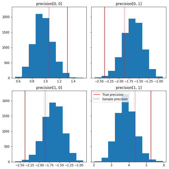
หากเราไม่มีวิธีแก้ปัญหาเชิงวิเคราะห์ นี่ก็เป็นเวลาที่จะต้องวิจารณ์แบบจำลองที่แท้จริง
ต่อไปนี้คือฮิสโทแกรมสั้นๆ บางส่วนของส่วนประกอบตัวอย่างที่สัมพันธ์กับความจริงพื้นๆ ของเรา (สีแดง) โปรดทราบว่าตัวอย่างถูกย่อจากค่าเมทริกซ์ความแม่นยำของตัวอย่างไปยังเมทริกซ์เอกลักษณ์ก่อนหน้านี้
fig, axes = plt.subplots(2, 2, sharey=True)
fig.set_size_inches(8, 8)
for i in range(2):
  for j in range(2):
    ax = axes[i, j]
    ax.hist(precision_samples_reshaped[:, i, j])
    ax.axvline(true_precision[i, j], color='red',
               label='True precision')
    ax.axvline(sample_precision[i, j], color='red', linestyle=':',
               label='Sample precision')
    ax.set_title('precision[%d, %d]' % (i, j))
plt.tight_layout()
plt.legend()
plt.show()
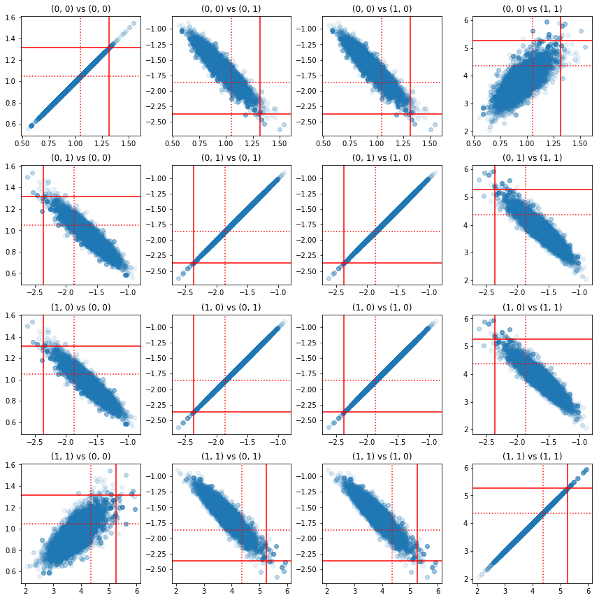
แผนภาพกระจายของคู่ของส่วนประกอบที่มีความแม่นยำแสดงให้เห็นว่าเนื่องจากโครงสร้างสหสัมพันธ์ของส่วนหลัง ค่าส่วนหลังที่แท้จริงไม่น่าจะเป็นไปได้อย่างที่ปรากฏจากส่วนขอบด้านบน
fig, axes = plt.subplots(4, 4)
fig.set_size_inches(12, 12)
for i1 in range(2):
  for j1 in range(2):
    index1 = 2 * i1 + j1
    for i2 in range(2):
      for j2 in range(2):
        index2 = 2 * i2 + j2
        ax = axes[index1, index2]
        ax.scatter(precision_samples_reshaped[:, i1, j1],
                   precision_samples_reshaped[:, i2, j2], alpha=0.1)
        ax.axvline(true_precision[i1, j1], color='red')
        ax.axhline(true_precision[i2, j2], color='red')
        ax.axvline(sample_precision[i1, j1], color='red', linestyle=':')
        ax.axhline(sample_precision[i2, j2], color='red', linestyle=':')
        ax.set_title('(%d, %d) vs (%d, %d)' % (i1, j1, i2, j2))
plt.tight_layout()
plt.show()
เวอร์ชัน 4: การสุ่มตัวอย่างพารามิเตอร์ที่จำกัดได้ง่ายขึ้น
Bijectors สุ่มตัวอย่างเมทริกซ์ที่มีความแม่นยำตรงไปตรงมา แต่มีการแปลงแบบแมนนวลเป็นและจากการแสดงที่ไม่มีข้อ จำกัด จำนวนพอสมควร มีวิธีที่ง่ายกว่านั้น!
TransformedTransitionKernel
TransformedTransitionKernel ลดความยุ่งยากในขั้นตอนนี้ มันห่อตัวเก็บตัวอย่างของคุณและจัดการการแปลงทั้งหมด ใช้เป็นอาร์กิวเมนต์รายการของ bijectors ที่จับคู่ค่าพารามิเตอร์ที่ไม่มีข้อจำกัดกับค่าที่จำกัด ดังนั้นที่นี่เราต้องผกผันของ precision_to_unconstrained bijector เราใช้ข้างต้น เราก็สามารถใช้ tfb.Invert(precision_to_unconstrained) แต่ที่จะเกี่ยวข้องกับการรับแปรผกผันของแปรผกผัน (TensorFlow ไม่เพียงพอที่สมาร์ทเพื่อลดความซับซ้อน tf.Invert(tf.Invert()) เพื่อ tf.Identity()) เพื่อแทนเรา จะเขียน bijector ใหม่
จำกัด bijector
# The bijector we need for the TransformedTransitionKernel is the inverse of
# the one we used above
unconstrained_to_precision = tfb.Chain([
    # step 3: take the product of Cholesky factors
    tfb.CholeskyOuterProduct(validate_args=VALIDATE_ARGS),
    # step 2: exponentiate the diagonals
    tfb.TransformDiagonal(tfb.Exp(validate_args=VALIDATE_ARGS)),
    # step 1: map a vector to a lower triangular matrix
    tfb.FillTriangular(validate_args=VALIDATE_ARGS),
])
# quick sanity check
m = [[1., 2.], [2., 8.]]
m_inv = unconstrained_to_precision.inverse(m).numpy()
m_fwd = unconstrained_to_precision.forward(m_inv).numpy()

print('m:\n', m)
print('unconstrained_to_precision.inverse(m):\n', m_inv)
print('forward(unconstrained_to_precision.inverse(m)):\n', m_fwd)
m:
 [[1.0, 2.0], [2.0, 8.0]]
unconstrained_to_precision.inverse(m):
 [0.6931472 2.        0.       ]
forward(unconstrained_to_precision.inverse(m)):
 [[1. 2.]
 [2. 8.]]
สุ่มตัวอย่างด้วย TransformedTransitionKernel
ด้วย TransformedTransitionKernel เราไม่ต้องทำแปลงคู่มือของพารามิเตอร์ของเรา ค่าเริ่มต้นและตัวอย่างของเราล้วนเป็นเมทริกซ์ที่มีความแม่นยำ เราแค่ต้องส่ง bijector ที่ไม่มีข้อจำกัดของเราไปยังเคอร์เนล และดูแลการเปลี่ยนแปลงทั้งหมด
@tf.function(autograph=False)
def sample():
  tf.random.set_seed(123)
  log_lik_fn = get_log_lik(my_data)

  # Tuning acceptance rates:
  dtype = np.float32
  num_burnin_iter = 3000
  num_warmup_iter = int(0.8 * num_burnin_iter)
  num_chain_iter = 2500

  # Set the target average acceptance ratio for the HMC as suggested by
  # Beskos et al. (2013):
  # https://projecteuclid.org/download/pdfview_1/euclid.bj/1383661192
  target_accept_rate = 0.651

  # Initialize the HMC sampler.
  hmc = tfp.mcmc.HamiltonianMonteCarlo(
      target_log_prob_fn=log_lik_fn,
      step_size=0.01,
      num_leapfrog_steps=3)

  ttk = tfp.mcmc.TransformedTransitionKernel(
      inner_kernel=hmc, bijector=unconstrained_to_precision)

  # Adapt the step size using standard adaptive MCMC procedure. See Section 4.2
  # of Andrieu and Thoms (2008):
  # http://www4.ncsu.edu/~rsmith/MA797V_S12/Andrieu08_AdaptiveMCMC_Tutorial.pdf
  adapted_kernel = tfp.mcmc.SimpleStepSizeAdaptation(
      inner_kernel=ttk,
      num_adaptation_steps=num_warmup_iter,
      target_accept_prob=target_accept_rate)

  states = tfp.mcmc.sample_chain(
      num_results=num_chain_iter,
      num_burnin_steps=num_burnin_iter,
      current_state=initial_values,
      kernel=adapted_kernel,
      trace_fn=None,
      parallel_iterations=1)
  # transform samples back to their constrained form
  return states

precision_samples  = sample()
กำลังตรวจสอบการบรรจบกัน
\(\hat{R}\) บรรจบเช็คดูดี!
r_hat = tfp.mcmc.potential_scale_reduction(precision_samples).numpy()
print(r_hat)
[[1.0013582 1.0019467]
 [1.0019467 1.0011805]]
เปรียบเทียบกับการวิเคราะห์หลัง
ลองตรวจสอบกับการวิเคราะห์หลังอีกครั้ง
# The output samples have shape [n_steps, n_chains, 2, 2]
# Flatten them to [n_steps * n_chains, 2, 2] via reshape:
precision_samples_reshaped = np.reshape(precision_samples, [-1, 2, 2])
print('True posterior mean:\n', posterior_mean)
print('Mean of samples:\n', np.mean(precision_samples_reshaped, axis=0))
True posterior mean:
 [[ 0.9641779 -1.6534661]
 [-1.6534661  3.8683164]]
Mean of samples:
 [[ 0.96687526 -1.6552585 ]
 [-1.6552585   3.867676  ]]
print('True posterior standard deviation:\n', posterior_sd)
print('Standard deviation of samples:\n', np.std(precision_samples_reshaped, axis=0))
True posterior standard deviation:
 [[0.13435492 0.25050813]
 [0.25050813 0.53903675]]
Standard deviation of samples:
 [[0.13329624 0.24913791]
 [0.24913791 0.53983927]]
การเพิ่มประสิทธิภาพ
ตอนนี้เรามีสิ่งต่าง ๆ ที่ทำงานแบบ end-to-end แล้ว มาทำเวอร์ชันที่ปรับให้เหมาะสมกันดีกว่า ความเร็วไม่สำคัญมากนักสำหรับตัวอย่างนี้ แต่เมื่อเมทริกซ์มีขนาดใหญ่ขึ้น การเพิ่มประสิทธิภาพบางอย่างจะสร้างความแตกต่างอย่างมาก
การปรับปรุงความเร็วครั้งใหญ่อย่างหนึ่งที่เราทำได้คือการปรับพารามิเตอร์ใหม่ในแง่ของการสลายตัวของ Cholesky เหตุผลก็คือฟังก์ชันความน่าจะเป็นของข้อมูลต้องการทั้งความแปรปรวนร่วมและเมทริกซ์ความแม่นยำ เมทริกซ์ผกผันมีราคาแพง (\(O(n^3)\) สำหรับ \(n \times n\) เมทริกซ์) และถ้าเรา parameterize ในแง่ของทั้งแปรปรวนหรือเมทริกซ์ที่มีความแม่นยำที่เราต้องทำเพื่อให้ได้ผกผันอื่น ๆ
ในฐานะที่เป็นเตือนจริงบวกที่ชัดเจน, สมมาตรเมทริกซ์ \(M\) สามารถย่อยสลายลงในผลิตภัณฑ์ของรูปแบบ \(M = L L^T\) ที่เมทริกซ์ \(L\) เป็นรูปสามเหลี่ยมที่ต่ำกว่าและมีเส้นทแยงมุมในเชิงบวก ได้รับการสลายตัว Cholesky ของ \(M\)เรามีประสิทธิภาพมากขึ้นสามารถได้รับทั้ง \(M\) (ผลิตภัณฑ์ของที่ต่ำกว่าและเมทริกซ์สามเหลี่ยมบน) และ \(M^{-1}\) (ผ่านกลับมาทดแทน) การแยกตัวประกอบของ Cholesky นั้นไม่ถูกในการคำนวณ แต่ถ้าเราสร้างพารามิเตอร์ในแง่ของปัจจัย Cholesky เราจำเป็นต้องคำนวณตัวประกอบ Choleksy ของค่าพารามิเตอร์เริ่มต้นเท่านั้น
การใช้การสลายตัวของ Cholesky ของเมทริกซ์ความแปรปรวนร่วม
TFP มีรุ่นของการกระจายปกติหลายตัวแปรเป็น MultivariateNormalTriL ที่ถูกแปรในแง่ของปัจจัย Cholesky ของเมทริกซ์ความแปรปรวนร่วม ดังนั้นถ้าเราต้องสร้างพารามิเตอร์ในรูปของปัจจัย Cholesky ของเมทริกซ์ความแปรปรวนร่วม เราสามารถคำนวณความน่าจะเป็นของบันทึกข้อมูลได้อย่างมีประสิทธิภาพ ความท้าทายคือการคำนวณความเป็นไปได้ของบันทึกก่อนหน้าที่มีประสิทธิภาพใกล้เคียงกัน
หากเรามีเวอร์ชันของการแจกแจง Wishart ผกผันที่ทำงานกับปัจจัย Cholesky ของกลุ่มตัวอย่าง เราก็พร้อมแล้ว อนิจจาเราไม่ได้ (แต่ทีมงานยินดีส่งโค้ด!) อีกทางเลือกหนึ่งคือ เราสามารถใช้เวอร์ชันของการแจกจ่าย Wishart ที่ทำงานร่วมกับปัจจัยของตัวอย่าง Cholesky ร่วมกับกลุ่มของ bijectors
ในขณะนี้ เราไม่มี bijectors สต็อกสองสามตัวที่จะทำให้สิ่งต่าง ๆ มีประสิทธิภาพจริงๆ แต่ฉันต้องการแสดงกระบวนการนี้เป็นแบบฝึกหัดและภาพประกอบที่มีประโยชน์เกี่ยวกับพลังของ bijectors ของ TFP
การกระจาย Wishart ที่ทำงานบนปัจจัย Cholesky
Wishart กระจายมีธงประโยชน์ input_output_cholesky ที่ระบุว่าเข้าและส่งออกการฝึกอบรมควรจะเป็นปัจจัย Cholesky การทำงานกับปัจจัย Cholesky มีประสิทธิภาพและเป็นข้อได้เปรียบเชิงตัวเลขมากกว่าเมทริกซ์เต็ม ซึ่งเป็นเหตุผลว่าทำไมจึงควรทำเช่นนี้ จุดสำคัญที่เกี่ยวกับความหมายของธง: มันเป็นเพียงข้อบ่งชี้ว่าเป็นตัวแทนของอินพุตและเอาต์พุตการกระจายควรเปลี่ยน - มันไม่ได้หมายความถึง reparameterization เต็มรูปแบบของการจัดจำหน่ายซึ่งจะเกี่ยวข้องกับการแก้ไขจาโคเบียนไป log_prob() การทำงาน. เราต้องการทำการกำหนดพารามิเตอร์ใหม่ทั้งหมด ดังนั้นเราจะสร้างการกระจายของเราเอง
# An optimized Wishart distribution that has been transformed to operate on
# Cholesky factors instead of full matrices.  Note that we gain a modest
# additional speedup by specifying the Cholesky factor of the scale matrix
# (i.e. by passing in the scale_tril parameter instead of scale).

class CholeskyWishart(tfd.TransformedDistribution):
  """Wishart distribution reparameterized to use Cholesky factors."""
  def __init__(self,
      df,
      scale_tril,
      validate_args=False,
      allow_nan_stats=True,
      name='CholeskyWishart'):
    # Wishart has a bunch of methods that we want to support but not
    # implement.  We'll subclass TransformedDistribution here to take care of
    # those.  We'll override the few for which speed is critical and implement
    # them with a separate Wishart for which input_output_cholesky=True
    super(CholeskyWishart, self).__init__(
        distribution=tfd.WishartTriL(
            df=df,
            scale_tril=scale_tril,
            input_output_cholesky=False,
            validate_args=validate_args,
            allow_nan_stats=allow_nan_stats),
        bijector=tfb.Invert(tfb.CholeskyOuterProduct()),
        validate_args=validate_args,
        name=name
    )
    # Here's the Cholesky distribution we'll use for log_prob() and sample()
    self.cholesky = tfd.WishartTriL(
        df=df,
        scale_tril=scale_tril,
        input_output_cholesky=True,
        validate_args=validate_args,
        allow_nan_stats=allow_nan_stats)

  def _log_prob(self, x):
    return (self.cholesky.log_prob(x) +
            self.bijector.inverse_log_det_jacobian(x, event_ndims=2))

  def _sample_n(self, n, seed=None):
    return self.cholesky._sample_n(n, seed)
# some checks
PRIOR_SCALE_CHOLESKY = np.linalg.cholesky(PRIOR_SCALE)

@tf.function(autograph=False)
def compute_log_prob(m):
  w_transformed = tfd.TransformedDistribution(
      tfd.WishartTriL(df=PRIOR_DF, scale_tril=PRIOR_SCALE_CHOLESKY),
      bijector=tfb.Invert(tfb.CholeskyOuterProduct()))
  w_optimized = CholeskyWishart(
      df=PRIOR_DF, scale_tril=PRIOR_SCALE_CHOLESKY)
  log_prob_transformed = w_transformed.log_prob(m)
  log_prob_optimized = w_optimized.log_prob(m)
  return log_prob_transformed, log_prob_optimized

for matrix in [np.eye(2, dtype=np.float32),
               np.array([[1., 0.], [2., 8.]], dtype=np.float32)]:
  log_prob_transformed, log_prob_optimized = [
      t.numpy() for t in compute_log_prob(matrix)]
  print('Transformed Wishart:', log_prob_transformed)
  print('Optimized Wishart', log_prob_optimized)
Transformed Wishart: -0.84889317
Optimized Wishart -0.84889317
Transformed Wishart: -99.269455
Optimized Wishart -99.269455
การสร้างการกระจาย Wishart ผกผัน
เราได้ของเราแปรปรวนเมทริกซ์ \(C\) ย่อยสลายเป็น \(C = L L^T\) ที่ \(L\) เป็นรูปสามเหลี่ยมที่ต่ำกว่าและมีเส้นทแยงมุมในเชิงบวก เราต้องการที่จะรู้ว่าน่าจะเป็นของ \(L\) ให้ที่ \(C \sim W^{-1}(\nu, V)\) ที่ \(W^{-1}\) คือการกระจายริชาร์ตผกผัน
การกระจายผกผันริชาร์ตมีคุณสมบัติที่ว่าถ้า \(C \sim W^{-1}(\nu, V)\)แล้วความแม่นยำเมทริกซ์ \(C^{-1} \sim W(\nu, V^{-1})\)ดังนั้นเราจะได้รับความน่าจะเป็นของ \(L\) ผ่าน TransformedDistribution ที่ใช้เป็นพารามิเตอร์การกระจายริชาร์ตและ bijector ที่แผนที่ปัจจัย Cholesky ของเมทริกซ์ที่มีความแม่นยำในการเป็นปัจจัย Cholesky ของสิ่งที่ตรงกันข้าม
ตรงไปตรงมา ( แต่ไม่ได้มีประสิทธิภาพสูง) วิธีการที่จะได้รับจากปัจจัย Cholesky ของ \(C^{-1}\) เพื่อ \(L\) คือการกลับปัจจัย Cholesky โดยกลับมาแก้แล้วขึ้นรูปเมทริกซ์ความแปรปรวนจากปัจจัยฤๅษีเหล่านี้และจากนั้นทำตัวประกอบ Cholesky .
ให้สลายตัว Cholesky ของ \(C^{-1} = M M^T\)\(M\) เป็นรูปสามเหลี่ยมที่ต่ำกว่าเพื่อให้เราสามารถกลับโดยใช้ MatrixInverseTriL bijector
การขึ้นรูป \(C\) จาก \(M^{-1}\) เป็นเพียงเล็กน้อยหากิน: \(C = (M M^T)^{-1} = M^{-T}M^{-1} = M^{-T} (M^{-T})^T\)\(M\) เป็นรูปสามเหลี่ยมที่ต่ำกว่าดังนั้น \(M^{-1}\) ยังจะเป็นรูปสามเหลี่ยมที่ต่ำกว่าและ \(M^{-T}\) จะเป็นรูปสามเหลี่ยมบน CholeskyOuterProduct() bijector เท่านั้นทำงานร่วมกับเมทริกซ์สามเหลี่ยมต่ำดังนั้นเราจึงไม่สามารถใช้งานได้ในรูปแบบ \(C\) จาก \(M^{-T}\)วิธีแก้ปัญหาของเราคือกลุ่มของ bijectors ที่เปลี่ยนแถวและคอลัมน์ของเมทริกซ์
โชคดีที่ตรรกะนี้จะห่อหุ้มใน CholeskyToInvCholesky bijector!
ผสมผสานทุกชิ้น
# verify that the bijector works
m = np.array([[1., 0.], [2., 8.]], dtype=np.float32)
c_inv = m.dot(m.T)
c = np.linalg.inv(c_inv)
c_chol = np.linalg.cholesky(c)
wishart_cholesky_to_iw_cholesky = tfb.CholeskyToInvCholesky()
w_fwd = wishart_cholesky_to_iw_cholesky.forward(m).numpy()

print('numpy =\n', c_chol)
print('bijector =\n', w_fwd)
numpy =
 [[ 1.0307764   0.        ]
 [-0.03031695  0.12126781]]
bijector =
 [[ 1.0307764   0.        ]
 [-0.03031695  0.12126781]]
การกระจายสินค้าครั้งสุดท้ายของเรา
Wishart ผกผันของเราทำงานบนปัจจัย Cholesky มีดังนี้:
inverse_wishart_cholesky = tfd.TransformedDistribution(
    distribution=CholeskyWishart(
        df=PRIOR_DF,
        scale_tril=np.linalg.cholesky(np.linalg.inv(PRIOR_SCALE))),
    bijector=tfb.CholeskyToInvCholesky())
เรามี Wishart ผกผัน แต่มันค่อนข้างช้าเพราะเราต้องสลาย Cholesky ใน bijector กลับไปที่การกำหนดพารามิเตอร์เมทริกซ์ที่แม่นยำและดูว่าเราสามารถทำอะไรได้บ้างเพื่อการเพิ่มประสิทธิภาพ
เวอร์ชันสุดท้าย (!): ใช้การสลายตัวของ Cholesky ของเมทริกซ์ความแม่นยำ
แนวทางอื่นคือการทำงานกับปัจจัย Cholesky ของเมทริกซ์ความแม่นยำ ในที่นี้ ฟังก์ชันความน่าจะเป็นก่อนหน้านั้นคำนวณได้ง่าย แต่ฟังก์ชันความน่าจะเป็นของการบันทึกข้อมูลใช้งานได้มากกว่า เนื่องจาก TFP ไม่มีเวอร์ชันของตัวแปรหลายตัวแปรปกติที่ตั้งค่าพารามิเตอร์ด้วยความแม่นยำ
ปรับปรุงโอกาสในการบันทึกก่อนหน้า
เราใช้ CholeskyWishart กระจายเราสร้างดังกล่าวข้างต้นที่จะสร้างก่อน
# Our new prior.
PRIOR_SCALE_CHOLESKY = np.linalg.cholesky(PRIOR_SCALE)

def log_lik_prior_cholesky(precisions_cholesky):
  rv_precision = CholeskyWishart(
      df=PRIOR_DF,
      scale_tril=PRIOR_SCALE_CHOLESKY,
      validate_args=VALIDATE_ARGS,
      allow_nan_stats=ALLOW_NAN_STATS)
  return rv_precision.log_prob(precisions_cholesky)
# Check against the slower TF implementation and the NumPy implementation.
# Note that when comparing to NumPy, we need to add in the Jacobian correction.
precisions = [np.eye(2, dtype=np.float32),
              true_precision]
precisions_cholesky = np.stack([np.linalg.cholesky(m) for m in precisions])
precisions = np.stack(precisions)
lik_tf = log_lik_prior_cholesky(precisions_cholesky).numpy()
lik_tf_slow = tfd.TransformedDistribution(
    distribution=tfd.WishartTriL(
        df=PRIOR_DF, scale_tril=tf.linalg.cholesky(PRIOR_SCALE)),
    bijector=tfb.Invert(tfb.CholeskyOuterProduct())).log_prob(
    precisions_cholesky).numpy()
corrections = tfb.Invert(tfb.CholeskyOuterProduct()).inverse_log_det_jacobian(
    precisions_cholesky, event_ndims=2).numpy()
n = precisions.shape[0]

for i in range(n):
  print(i)
  print('numpy:', log_lik_prior_numpy(precisions[i]) + corrections[i])
  print('tensorflow slow:', lik_tf_slow[i])
  print('tensorflow fast:', lik_tf[i])
0
numpy: -0.8488930160357633
tensorflow slow: -0.84889317
tensorflow fast: -0.84889317
1
numpy: -7.442875031036973
tensorflow slow: -7.442877
tensorflow fast: -7.442876
โอกาสในการบันทึกข้อมูลที่เหมาะสมที่สุด
We can use TFP's bijectors to build our own version of the multivariate normal. Here is the key idea:
Suppose I have a column vector \(X\) whose elements are iid samples of \(N(0, 1)\). We have \(\text{mean}(X) = 0\) and \(\text{cov}(X) = I\)
Now let \(Y = A X + b\). We have \(\text{mean}(Y) = b\) and \(\text{cov}(Y) = A A^T\)
Hence we can make vectors with mean \(b\) and covariance \(C\) using the affine transform \(Ax+b\) to vectors of iid standard Normal samples provided \(A A^T = C\). The Cholesky decomposition of \(C\) has the desired property. However, there are other solutions.
Let \(P = C^{-1}\) and let the Cholesky decomposition of \(P\) be \(B\), ie \(B B^T = P\). Now
\(P^{-1} = (B B^T)^{-1} = B^{-T} B^{-1} = B^{-T} (B^{-T})^T\)
So another way to get our desired mean and covariance is to use the affine transform \(Y=B^{-T}X + b\).
Our approach (courtesy of this notebook ):
- Use
tfd.Independent()to combine a batch of 1-DNormalrandom variables into a single multi-dimensional random variable. Thereinterpreted_batch_ndimsparameter forIndependent()specifies the number of batch dimensions that should be reinterpreted as event dimensions. In our case we create a 1-D batch of length 2 that we transform into a 1-D event of length 2, soreinterpreted_batch_ndims=1. - Apply a bijector to add the desired covariance:
tfb.Invert(tfb.ScaleMatvecTriL(scale_tril=precision_cholesky, adjoint=True)). Note that above we're multiplying our iid normal random variables by the transpose of the inverse of the Cholesky factor of the precision matrix \((B^{-T}X)\). Thetfb.Inverttakes care of inverting \(B\), and theadjoint=Trueflag performs the transpose. - Apply a bijector to add the desired offset:
tfb.Shift(shift=shift)Note that we have to do the shift as a separate step from the initial inverted affine transform because otherwise the inverted scale is applied to the shift (since the inverse of \(y=Ax+b\) is \(x=A^{-1}y - A^{-1}b\)).
class MVNPrecisionCholesky(tfd.TransformedDistribution):
  """Multivariate normal parameterized by loc and Cholesky precision matrix."""

  def __init__(self, loc, precision_cholesky, name=None):
    super(MVNPrecisionCholesky, self).__init__(
        distribution=tfd.Independent(
            tfd.Normal(loc=tf.zeros_like(loc),
                       scale=tf.ones_like(loc)),
            reinterpreted_batch_ndims=1),
        bijector=tfb.Chain([
            tfb.Shift(shift=loc),
            tfb.Invert(tfb.ScaleMatvecTriL(scale_tril=precision_cholesky,
                                  adjoint=True)),
        ]),
        name=name)
@tf.function(autograph=False)
def log_lik_data_cholesky(precisions_cholesky, replicated_data):
  n = tf.shape(precisions_cholesky)[0]  # number of precision matrices
  rv_data = MVNPrecisionCholesky(
      loc=tf.zeros([n, 2]),
      precision_cholesky=precisions_cholesky)
  return tf.reduce_sum(rv_data.log_prob(replicated_data), axis=0)
# check against the numpy implementation
true_precision_cholesky = np.linalg.cholesky(true_precision)
precisions = [np.eye(2, dtype=np.float32), true_precision]
precisions_cholesky = np.stack([np.linalg.cholesky(m) for m in precisions])
precisions = np.stack(precisions)
n = precisions_cholesky.shape[0]
replicated_data = np.tile(np.expand_dims(my_data, axis=1), reps=[1, 2, 1])
lik_tf = log_lik_data_cholesky(precisions_cholesky, replicated_data).numpy()

for i in range(n):
  print(i)
  print('numpy:', log_lik_data_numpy(precisions[i], my_data))
  print('tensorflow:', lik_tf[i])
0
numpy: -430.71218815801365
tensorflow: -430.71207
1
numpy: -280.81822950593767
tensorflow: -280.81824
Combined log likelihood function
Now we combine our prior and data log likelihood functions in a closure.
def get_log_lik_cholesky(data, n_chains=1):
  # The data argument that is passed in will be available to the inner function
  # below so it doesn't have to be passed in as a parameter.
  replicated_data = np.tile(np.expand_dims(data, axis=1), reps=[1, n_chains, 1])

  @tf.function(autograph=False)
  def _log_lik_cholesky(precisions_cholesky):
    return (log_lik_data_cholesky(precisions_cholesky, replicated_data) +
            log_lik_prior_cholesky(precisions_cholesky))

  return _log_lik_cholesky
Constraining bijector
Our samples are constrained to be valid Cholesky factors, which means they must be lower triangular matrices with positive diagonals. The TransformedTransitionKernel needs a bijector that maps unconstrained tensors to/from tensors with our desired constraints. We've removed the Cholesky decomposition from the bijector's inverse, which speeds things up.
unconstrained_to_precision_cholesky = tfb.Chain([
    # step 2: exponentiate the diagonals
    tfb.TransformDiagonal(tfb.Exp(validate_args=VALIDATE_ARGS)),
    # step 1: expand the vector to a lower triangular matrix
    tfb.FillTriangular(validate_args=VALIDATE_ARGS),
])
# some checks
inv = unconstrained_to_precision_cholesky.inverse(precisions_cholesky).numpy()
fwd = unconstrained_to_precision_cholesky.forward(inv).numpy()
print('precisions_cholesky:\n', precisions_cholesky)
print('\ninv:\n', inv)
print('\nfwd(inv):\n', fwd)
precisions_cholesky:
 [[[ 1.         0.       ]
  [ 0.         1.       ]]

 [[ 1.1470785  0.       ]
  [-2.0647411  1.0000004]]]

inv:
 [[ 0.0000000e+00  0.0000000e+00  0.0000000e+00]
 [ 3.5762781e-07 -2.0647411e+00  1.3721828e-01]]

fwd(inv):
 [[[ 1.         0.       ]
  [ 0.         1.       ]]

 [[ 1.1470785  0.       ]
  [-2.0647411  1.0000004]]]
Initial values
We generate a tensor of initial values. We're working with Cholesky factors, so we generate some Cholesky factor initial values.
# The number of chains is determined by the shape of the initial values.
# Here we'll generate 3 chains, so we'll need a tensor of 3 initial values.
N_CHAINS = 3

np.random.seed(123)

initial_values_cholesky = []
for i in range(N_CHAINS):
  initial_values_cholesky.append(np.array(
      [[0.5 + np.random.uniform(), 0.0],
       [-0.5 + np.random.uniform(), 0.5 + np.random.uniform()]],
      dtype=np.float32))
initial_values_cholesky = np.stack(initial_values_cholesky)
Sampling
We sample N_CHAINS chains using the TransformedTransitionKernel .
@tf.function(autograph=False)
def sample():
  tf.random.set_seed(123)
  log_lik_fn = get_log_lik_cholesky(my_data)

  # Tuning acceptance rates:
  dtype = np.float32
  num_burnin_iter = 3000
  num_warmup_iter = int(0.8 * num_burnin_iter)
  num_chain_iter = 2500

  # Set the target average acceptance ratio for the HMC as suggested by
  # Beskos et al. (2013):
  # https://projecteuclid.org/download/pdfview_1/euclid.bj/1383661192
  target_accept_rate = 0.651

  # Initialize the HMC sampler.
  hmc = tfp.mcmc.HamiltonianMonteCarlo(
      target_log_prob_fn=log_lik_fn,
      step_size=0.01,
      num_leapfrog_steps=3)

  ttk = tfp.mcmc.TransformedTransitionKernel(
      inner_kernel=hmc, bijector=unconstrained_to_precision_cholesky)

  # Adapt the step size using standard adaptive MCMC procedure. See Section 4.2
  # of Andrieu and Thoms (2008):
  # http://www4.ncsu.edu/~rsmith/MA797V_S12/Andrieu08_AdaptiveMCMC_Tutorial.pdf
  adapted_kernel = tfp.mcmc.SimpleStepSizeAdaptation(
      inner_kernel=ttk,
      num_adaptation_steps=num_warmup_iter,
      target_accept_prob=target_accept_rate)

  states = tfp.mcmc.sample_chain(
      num_results=num_chain_iter,
      num_burnin_steps=num_burnin_iter,
      current_state=initial_values,
      kernel=adapted_kernel,
      trace_fn=None,
      parallel_iterations=1)
  # transform samples back to their constrained form
  samples = tf.linalg.matmul(states, states, transpose_b=True)
  return samples

precision_samples = sample()
Convergence check
A quick convergence check looks good:
r_hat = tfp.mcmc.potential_scale_reduction(precision_samples).numpy()
print(r_hat)
[[1.0013583 1.0019467]
 [1.0019467 1.0011804]]
Comparing results to the analytic posterior
# The output samples have shape [n_steps, n_chains, 2, 2]
# Flatten them to [n_steps * n_chains, 2, 2] via reshape:
precision_samples_reshaped = np.reshape(precision_samples, newshape=[-1, 2, 2])
And again, the sample means and standard deviations match those of the analytic posterior.
print('True posterior mean:\n', posterior_mean)
print('Mean of samples:\n', np.mean(precision_samples_reshaped, axis=0))
True posterior mean:
 [[ 0.9641779 -1.6534661]
 [-1.6534661  3.8683164]]
Mean of samples:
 [[ 0.9668749 -1.6552604]
 [-1.6552604  3.8676758]]
print('True posterior standard deviation:\n', posterior_sd)
print('Standard deviation of samples:\n', np.std(precision_samples_reshaped, axis=0))
True posterior standard deviation:
 [[0.13435492 0.25050813]
 [0.25050813 0.53903675]]
Standard deviation of samples:
 [[0.13329637 0.24913797]
 [0.24913797 0.53983945]]
Ok, all done! We've got our optimized sampler working.