สวัสดีชาวโลกมากมาย

ดูบน TensorFlow.org

ทำงานใน Google Colab

ดูแหล่งที่มาบน GitHub

ดาวน์โหลดโน๊ตบุ๊ค

บทช่วยสอนนี้แสดงให้เห็นว่าโครงข่ายประสาทเทียมแบบคลาสสิกสามารถเรียนรู้วิธีแก้ไขข้อผิดพลาดในการสอบเทียบ qubit ได้อย่างไร แนะนำ Cirq ซึ่งเป็นเฟรมเวิร์ก Python เพื่อสร้าง แก้ไข และเรียกใช้วงจร Noisy Intermediate Scale Quantum (NISQ) และสาธิตวิธีที่ Cirq เชื่อมต่อกับ TensorFlow Quantum

ติดตั้ง

pip install tensorflow==2.7.0

ติดตั้ง TensorFlow Quantum:

pip install tensorflow-quantum

# Update package resources to account for version changes.
import importlib, pkg_resources
importlib.reload(pkg_resources)

<module 'pkg_resources' from '/tmpfs/src/tf_docs_env/lib/python3.7/site-packages/pkg_resources/__init__.py'>

ตอนนี้นำเข้า TensorFlow และการพึ่งพาโมดูล:

import tensorflow as tf
import tensorflow_quantum as tfq

import cirq
import sympy
import numpy as np

# visualization tools
%matplotlib inline
import matplotlib.pyplot as plt
from cirq.contrib.svg import SVGCircuit

2022-02-04 12:27:31.677071: E tensorflow/stream_executor/cuda/cuda_driver.cc:271] failed call to cuInit: CUDA_ERROR_NO_DEVICE: no CUDA-capable device is detected

1. พื้นฐาน

1.1 Cirq และวงจรควอนตัมแบบกำหนดพารามิเตอร์

ก่อนสำรวจ TensorFlow Quantum (TFQ) มาดูข้อมูลเบื้องต้นเกี่ยวกับ Cirq กันก่อน Cirq เป็นไลบรารี Python สำหรับการคำนวณควอนตัมจาก Google คุณใช้มันเพื่อกำหนดวงจร รวมถึงเกตแบบคงที่และแบบกำหนดพารามิเตอร์

Cirq ใช้สัญลักษณ์ SymPy เพื่อแสดงพารามิเตอร์อิสระ

a, b = sympy.symbols('a b')

รหัสต่อไปนี้สร้างวงจรสองบิตโดยใช้พารามิเตอร์ของคุณ:

# Create two qubits
q0, q1 = cirq.GridQubit.rect(1, 2)

# Create a circuit on these qubits using the parameters you created above.
circuit = cirq.Circuit(
    cirq.rx(a).on(q0),
    cirq.ry(b).on(q1), cirq.CNOT(control=q0, target=q1))

SVGCircuit(circuit)

findfont: Font family ['Arial'] not found. Falling back to DejaVu Sans.

ในการประเมินวงจร คุณสามารถใช้อินเทอร์เฟซ cirq.Simulator คุณแทนที่พารามิเตอร์อิสระในวงจรด้วยตัวเลขเฉพาะโดยส่งผ่านวัตถุ cirq.ParamResolver รหัสต่อไปนี้คำนวณเอาต์พุตเวกเตอร์สถานะดิบของวงจรพารามิเตอร์ของคุณ:

# Calculate a state vector with a=0.5 and b=-0.5.
resolver = cirq.ParamResolver({a: 0.5, b: -0.5})
output_state_vector = cirq.Simulator().simulate(circuit, resolver).final_state_vector
output_state_vector

array([ 0.9387913 +0.j        , -0.23971277+0.j        ,

        0.        +0.06120872j,  0.        -0.23971277j], dtype=complex64)

ตัวยึดตำแหน่ง22

เวกเตอร์สถานะไม่สามารถเข้าถึงได้โดยตรงนอกการจำลอง (สังเกตตัวเลขที่ซับซ้อนในผลลัพธ์ด้านบน) เพื่อให้มีความสมจริงทางกายภาพ คุณต้องระบุการวัด ซึ่งจะแปลงเวกเตอร์สถานะเป็นจำนวนจริงที่คอมพิวเตอร์คลาสสิกสามารถเข้าใจได้ Cirq ระบุการวัดโดยใช้การรวมกันของตัว ดำเนินการ Pauli \(\hat{X}\), \(\hat{Y}\)และ \(\hat{Z}\)ดังภาพประกอบ โค้ดต่อไปนี้วัด \(\hat{Z}_0\) และ \(\frac{1}{2}\hat{Z}_0 + \hat{X}_1\) บนเวกเตอร์สถานะที่คุณเพิ่งจำลอง:

z0 = cirq.Z(q0)

qubit_map={q0: 0, q1: 1}

z0.expectation_from_state_vector(output_state_vector, qubit_map).real

0.8775825500488281

z0x1 = 0.5 * z0 + cirq.X(q1)

z0x1.expectation_from_state_vector(output_state_vector, qubit_map).real

-0.04063427448272705

1.2 วงจรควอนตัมเป็นตัวเทนเซอร์

TensorFlow Quantum (TFQ) จัดเตรียม tfq.convert_to_tensor ซึ่งเป็นฟังก์ชันที่แปลงวัตถุ Cirq เป็นเมตริกซ์ สิ่งนี้ทำให้คุณสามารถส่งอ็อบเจ็กต์ Cirq ไปยัง เลเยอร์ค วอนตัมและ quantum ops ของเรา ฟังก์ชันนี้สามารถเรียกใช้ได้ในรายการหรืออาร์เรย์ของ Cirq Circuits และ Cirq Paulis:

# Rank 1 tensor containing 1 circuit.
circuit_tensor = tfq.convert_to_tensor([circuit])

print(circuit_tensor.shape)
print(circuit_tensor.dtype)

(1,)
<dtype: 'string'>

สิ่งนี้เข้ารหัสอ็อบเจ็กต์ Cirq เป็นเทนเซอร์ tf.string ที่การดำเนินการ tfq ถอดรหัสตามต้องการ

# Rank 1 tensor containing 2 Pauli operators.
pauli_tensor = tfq.convert_to_tensor([z0, z0x1])
pauli_tensor.shape

TensorShape([2])

1.3 การจำลองวงจรแบตช์

TFQ มีวิธีการคำนวณค่าความคาดหวัง ตัวอย่าง และเวกเตอร์สถานะ สำหรับตอนนี้ มาเน้นที่ ค่าความคาดหวัง

อินเทอร์เฟซระดับสูงสุดสำหรับการคำนวณค่าความคาดหวังคือเลเยอร์ tfq.layers.Expectation ซึ่งเป็น tf.keras.Layer ในรูปแบบที่ง่ายที่สุด เลเยอร์นี้เทียบเท่ากับการจำลองวงจรแบบกำหนดพารามิเตอร์บน cirq.ParamResolvers หลายตัว ; อย่างไรก็ตาม TFQ อนุญาตให้ทำแบทช์ตามความหมายของ TensorFlow และวงจรถูกจำลองโดยใช้รหัส C ++ ที่มีประสิทธิภาพ

สร้างชุดค่าเพื่อแทนที่พารามิเตอร์ a และ b ของเรา:

batch_vals = np.array(np.random.uniform(0, 2 * np.pi, (5, 2)), dtype=np.float32)

การประมวลผลวงจรแบบแบตช์เหนือค่าพารามิเตอร์ใน Cirq ต้องใช้การวนซ้ำ:

cirq_results = []
cirq_simulator = cirq.Simulator()

for vals in batch_vals:
    resolver = cirq.ParamResolver({a: vals[0], b: vals[1]})
    final_state_vector = cirq_simulator.simulate(circuit, resolver).final_state_vector
    cirq_results.append(
        [z0.expectation_from_state_vector(final_state_vector, {
            q0: 0,
            q1: 1
        }).real])

print('cirq batch results: \n {}'.format(np.array(cirq_results)))

cirq batch results: 
 [[-0.66652703]
 [ 0.49764055]
 [ 0.67326665]
 [-0.95549959]
 [-0.81297827]]

ตัวยึดตำแหน่ง33

การดำเนินการเดียวกันนี้ทำให้ง่ายขึ้นใน TFQ:

tfq.layers.Expectation()(circuit,
                         symbol_names=[a, b],
                         symbol_values=batch_vals,
                         operators=z0)

<tf.Tensor: shape=(5, 1), dtype=float32, numpy=
array([[-0.666526  ],
       [ 0.49764216],
       [ 0.6732664 ],
       [-0.9554999 ],
       [-0.8129788 ]], dtype=float32)>

2. การเพิ่มประสิทธิภาพควอนตัมคลาสสิกแบบไฮบริด

ตอนนี้คุณได้เห็นพื้นฐานแล้ว ลองใช้ TensorFlow Quantum เพื่อสร้าง โครงข่ายประสาทควอนตัมคลาสสิกแบบไฮบริด คุณจะฝึกโครงข่ายประสาทแบบคลาสสิกเพื่อควบคุม qubit เดียว การควบคุมจะได้รับการปรับให้เหมาะสมเพื่อเตรียม qubit อย่างถูกต้องในสถานะ 0 หรือ 1 เพื่อเอาชนะข้อผิดพลาดในการสอบเทียบอย่างเป็นระบบที่จำลองขึ้น รูปนี้แสดงสถาปัตยกรรม:

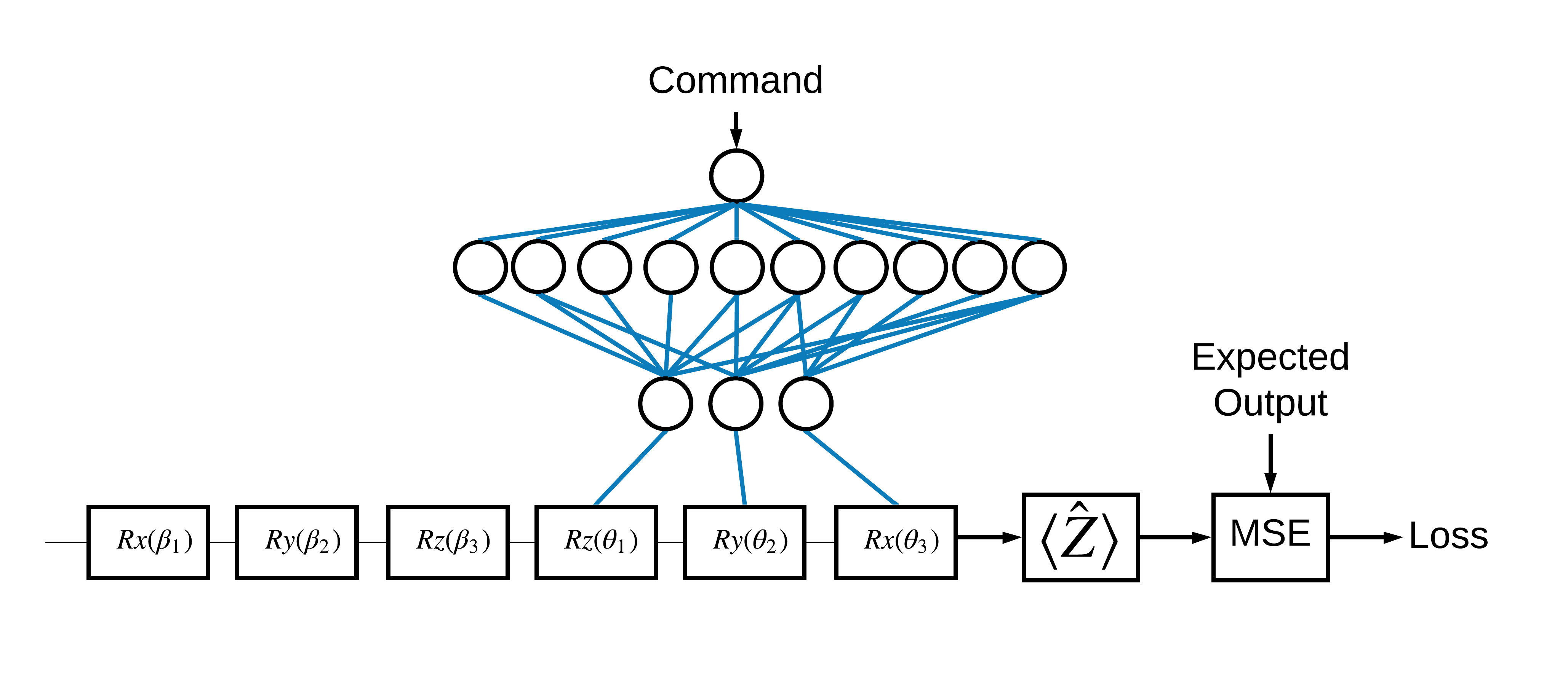
แม้จะไม่มีโครงข่ายประสาทเทียม แต่ก็เป็นปัญหาที่ตรงไปตรงมาในการแก้ไข แต่ธีมก็คล้ายกับปัญหาการควบคุมควอนตัมจริงที่คุณอาจแก้ไขโดยใช้ TFQ มันแสดงให้เห็นตัวอย่างแบบ end-to-end ของการคำนวณควอนตัมคลาสสิกโดยใช้ tfq.layers.ControlledPQC (Parametrized Quantum Circuit) ภายใน tf.keras.Model

สำหรับการใช้งานบทช่วยสอนนี้ สถาปัตยกรรมนี้แบ่งออกเป็น 3 ส่วน:

• วงจรอินพุทหรือวงจร ดาต้าพอยท์ : \(R\) ท 3 ตัวแรก
• วงจรควบคุม : เกท \(R\) อีก 3 เกท
• ตัวควบคุม : โครงข่ายประสาทเทียมแบบคลาสสิกที่ตั้งค่าพารามิเตอร์ของวงจรควบคุม

2.1 นิยามวงจรควบคุม

กำหนดการหมุนบิตเดียวที่เรียนรู้ได้ ดังที่แสดงในรูปด้านบน สิ่งนี้จะสอดคล้องกับวงจรควบคุมของเรา

# Parameters that the classical NN will feed values into.
control_params = sympy.symbols('theta_1 theta_2 theta_3')

# Create the parameterized circuit.
qubit = cirq.GridQubit(0, 0)
model_circuit = cirq.Circuit(
    cirq.rz(control_params[0])(qubit),
    cirq.ry(control_params[1])(qubit),
    cirq.rx(control_params[2])(qubit))

SVGCircuit(model_circuit)

2.2 ตัวควบคุม

ตอนนี้กำหนดเครือข่ายคอนโทรลเลอร์:

# The classical neural network layers.
controller = tf.keras.Sequential([
    tf.keras.layers.Dense(10, activation='elu'),
    tf.keras.layers.Dense(3)
])

ด้วยชุดคำสั่ง คอนโทรลเลอร์จะส่งสัญญาณควบคุมสำหรับวงจรควบคุม

คอนโทรลเลอร์ถูกเตรียมใช้งานแบบสุ่ม ดังนั้นเอาต์พุตเหล่านี้จึงยังไม่มีประโยชน์

controller(tf.constant([[0.0],[1.0]])).numpy()

array([[0.        , 0.        , 0.        ],
       [0.5815686 , 0.21376055, 0.57181627]], dtype=float32)

ตัวยึดตำแหน่ง39

2.3 เชื่อมต่อคอนโทรลเลอร์กับวงจร

ใช้ tfq เพื่อเชื่อมต่อคอนโทรลเลอร์กับวงจรควบคุมเป็น keras.Model เดียว

ดูคู่มือ Keras Functional API สำหรับข้อมูลเพิ่มเติมเกี่ยวกับรูปแบบการกำหนดรูปแบบนี้

ขั้นแรกให้กำหนดอินพุตให้กับโมเดล:

# This input is the simulated miscalibration that the model will learn to correct.
circuits_input = tf.keras.Input(shape=(),
                                # The circuit-tensor has dtype `tf.string` 
                                dtype=tf.string,
                                name='circuits_input')

# Commands will be either `0` or `1`, specifying the state to set the qubit to.
commands_input = tf.keras.Input(shape=(1,),
                                dtype=tf.dtypes.float32,
                                name='commands_input')

ถัดไป ใช้การดำเนินการกับอินพุตเหล่านั้น เพื่อกำหนดการคำนวณ

dense_2 = controller(commands_input)

# TFQ layer for classically controlled circuits.
expectation_layer = tfq.layers.ControlledPQC(model_circuit,
                                             # Observe Z
                                             operators = cirq.Z(qubit))
expectation = expectation_layer([circuits_input, dense_2])

ตอนนี้ทำแพ็กเกจการคำนวณนี้เป็น tf.keras.Model :

# The full Keras model is built from our layers.
model = tf.keras.Model(inputs=[circuits_input, commands_input],
                       outputs=expectation)

สถาปัตยกรรมเครือข่ายระบุโดยพล็อตของโมเดลด้านล่าง เปรียบเทียบพล็อตโมเดลนี้กับไดอะแกรมสถาปัตยกรรมเพื่อตรวจสอบความถูกต้อง

tf.keras.utils.plot_model(model, show_shapes=True, dpi=70)

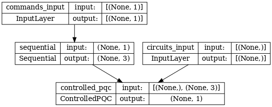
โมเดลนี้รับอินพุตสองอินพุต: คำสั่งสำหรับคอนโทรลเลอร์ และวงจรอินพุตที่เอาต์พุตที่คอนโทรลเลอร์พยายามแก้ไข

2.4 ชุดข้อมูล

โมเดลพยายามแสดงผลค่าการวัดที่ถูกต้องของ \(\hat{Z}\) สำหรับแต่ละคำสั่ง คำสั่งและค่าที่ถูกต้องกำหนดไว้ด้านล่าง

# The command input values to the classical NN.
commands = np.array([[0], [1]], dtype=np.float32)

# The desired Z expectation value at output of quantum circuit.
expected_outputs = np.array([[1], [-1]], dtype=np.float32)

นี่ไม่ใช่ชุดข้อมูลการฝึกอบรมทั้งหมดสำหรับงานนี้ แต่ละจุดข้อมูลในชุดข้อมูลยังต้องการวงจรอินพุตด้วย

2.4 นิยามวงจรอินพุต

วงจรอินพุตด้านล่างกำหนดการปรับเทียบมาตรฐานแบบสุ่มที่โมเดลจะได้เรียนรู้การแก้ไข

random_rotations = np.random.uniform(0, 2 * np.pi, 3)
noisy_preparation = cirq.Circuit(
  cirq.rx(random_rotations[0])(qubit),
  cirq.ry(random_rotations[1])(qubit),
  cirq.rz(random_rotations[2])(qubit)
)
datapoint_circuits = tfq.convert_to_tensor([
  noisy_preparation
] * 2)  # Make two copied of this circuit

มีวงจรสองชุด หนึ่งชุดสำหรับแต่ละจุดข้อมูล

datapoint_circuits.shape

TensorShape([2])

2.5 การฝึกอบรม

ด้วยอินพุตที่กำหนด คุณสามารถทดสอบรันโมเดล tfq ได้

model([datapoint_circuits, commands]).numpy()

array([[0.95853525],
       [0.6272128 ]], dtype=float32)

ในตอนนี้ ให้เรียกใช้กระบวนการฝึกอบรมมาตรฐานเพื่อปรับค่าเหล่านี้ให้เป็นค่าที่ expected_outputs

optimizer = tf.keras.optimizers.Adam(learning_rate=0.05)
loss = tf.keras.losses.MeanSquaredError()
model.compile(optimizer=optimizer, loss=loss)
history = model.fit(x=[datapoint_circuits, commands],
                    y=expected_outputs,
                    epochs=30,
                    verbose=0)

plt.plot(history.history['loss'])
plt.title("Learning to Control a Qubit")
plt.xlabel("Iterations")
plt.ylabel("Error in Control")
plt.show()

ตัวยึดตำแหน่ง51

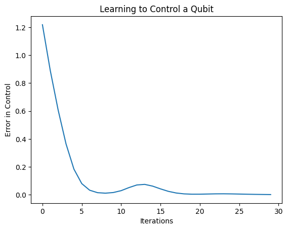
จากโครงเรื่องนี้ คุณจะเห็นว่าโครงข่ายประสาทเทียมได้เรียนรู้ที่จะเอาชนะการปรับเทียบผิดระบบอย่างเป็นระบบ

2.6 ตรวจสอบผลลัพธ์

ตอนนี้ใช้แบบจำลองที่ได้รับการฝึกอบรมเพื่อแก้ไขข้อผิดพลาดในการสอบเทียบ qubit ด้วย Cirq:

def check_error(command_values, desired_values):
  """Based on the value in `command_value` see how well you could prepare
  the full circuit to have `desired_value` when taking expectation w.r.t. Z."""
  params_to_prepare_output = controller(command_values).numpy()
  full_circuit = noisy_preparation + model_circuit

  # Test how well you can prepare a state to get expectation the expectation
  # value in `desired_values`
  for index in [0, 1]:
    state = cirq_simulator.simulate(
        full_circuit,
        {s:v for (s,v) in zip(control_params, params_to_prepare_output[index])}
    ).final_state_vector
    expt = cirq.Z(qubit).expectation_from_state_vector(state, {qubit: 0}).real
    print(f'For a desired output (expectation) of {desired_values[index]} with'
          f' noisy preparation, the controller\nnetwork found the following '
          f'values for theta: {params_to_prepare_output[index]}\nWhich gives an'
          f' actual expectation of: {expt}\n')


check_error(commands, expected_outputs)

For a desired output (expectation) of [1.] with noisy preparation, the controller
network found the following values for theta: [-0.6788422   0.3395225  -0.59394693]
Which gives an actual expectation of: 0.9171845316886902

For a desired output (expectation) of [-1.] with noisy preparation, the controller
network found the following values for theta: [-5.203663   -0.29528576  3.2887425 ]
Which gives an actual expectation of: -0.9511058330535889

ตัวยึดตำแหน่ง53

ค่าของฟังก์ชันการสูญเสียระหว่างการฝึกจะให้แนวคิดคร่าวๆ ว่าแบบจำลองเรียนรู้ได้ดีเพียงใด ยิ่งการสูญเสียต่ำเท่าใด ค่าความคาดหวังในเซลล์ด้านบนก็จะยิ่งใกล้ที่ต้องการที่ต้องการ desired_values ถ้าคุณไม่กังวลเกี่ยวกับค่าพารามิเตอร์ คุณสามารถตรวจสอบผลลัพธ์จากด้านบนได้ตลอดเวลาโดยใช้ tfq :

model([datapoint_circuits, commands])

<tf.Tensor: shape=(2, 1), dtype=float32, numpy=
array([[ 0.91718477],
       [-0.9511056 ]], dtype=float32)>

ตัวยึดตำแหน่ง55

3 การเรียนรู้เพื่อเตรียมลักษณะเฉพาะของตัวดำเนินการต่างๆ

ทางเลือกของ \(\pm \hat{Z}\) ลักษณะเฉพาะที่สอดคล้องกับ 1 และ 0 เป็นไปตามอำเภอใจ คุณสามารถมีเพียงแค่ 1 ที่ต้องการเพื่อให้สอดคล้องกับ \(+ \hat{Z}\) eigenstate และ 0 เพื่อให้สอดคล้องกับ \(-\hat{X}\) eigenstate วิธีหนึ่งในการบรรลุสิ่งนี้คือโดยการระบุตัวดำเนินการวัดที่แตกต่างกันสำหรับแต่ละคำสั่ง ดังที่แสดงในรูปด้านล่าง:

สิ่งนี้ต้องใช้ tfq.layers.Expectation ตอนนี้ข้อมูลที่คุณป้อนได้เติบโตขึ้นจนมีสามอ็อบเจ็กต์ ได้แก่ วงจร คำสั่ง และโอเปอเรเตอร์ ผลลัพธ์ยังคงเป็นค่าที่คาดหวัง

3.1 นิยามโมเดลใหม่

มาดูแบบจำลองเพื่อทำงานนี้ให้สำเร็จ:

# Define inputs.
commands_input = tf.keras.layers.Input(shape=(1),
                                       dtype=tf.dtypes.float32,
                                       name='commands_input')
circuits_input = tf.keras.Input(shape=(),
                                # The circuit-tensor has dtype `tf.string` 
                                dtype=tf.dtypes.string,
                                name='circuits_input')
operators_input = tf.keras.Input(shape=(1,),
                                 dtype=tf.dtypes.string,
                                 name='operators_input')

นี่คือเครือข่ายคอนโทรลเลอร์:

# Define classical NN.
controller = tf.keras.Sequential([
    tf.keras.layers.Dense(10, activation='elu'),
    tf.keras.layers.Dense(3)
])

รวมวงจรและคอนโทรลเลอร์เป็น keras.Model เดียวโดยใช้ tfq :

dense_2 = controller(commands_input)

# Since you aren't using a PQC or ControlledPQC you must append
# your model circuit onto the datapoint circuit tensor manually.
full_circuit = tfq.layers.AddCircuit()(circuits_input, append=model_circuit)
expectation_output = tfq.layers.Expectation()(full_circuit,
                                              symbol_names=control_params,
                                              symbol_values=dense_2,
                                              operators=operators_input)

# Contruct your Keras model.
two_axis_control_model = tf.keras.Model(
    inputs=[circuits_input, commands_input, operators_input],
    outputs=[expectation_output])

3.2 ชุดข้อมูล

ตอนนี้คุณจะรวมโอเปอเรเตอร์ที่คุณต้องการวัดสำหรับแต่ละจุดข้อมูลที่คุณจัดหาสำหรับ model_circuit :

# The operators to measure, for each command.
operator_data = tfq.convert_to_tensor([[cirq.X(qubit)], [cirq.Z(qubit)]])

# The command input values to the classical NN.
commands = np.array([[0], [1]], dtype=np.float32)

# The desired expectation value at output of quantum circuit.
expected_outputs = np.array([[1], [-1]], dtype=np.float32)

3.3 การฝึกอบรม

ตอนนี้คุณมีอินพุตและเอาต์พุตใหม่แล้ว คุณสามารถฝึกได้อีกครั้งโดยใช้ keras

optimizer = tf.keras.optimizers.Adam(learning_rate=0.05)
loss = tf.keras.losses.MeanSquaredError()

two_axis_control_model.compile(optimizer=optimizer, loss=loss)

history = two_axis_control_model.fit(
    x=[datapoint_circuits, commands, operator_data],
    y=expected_outputs,
    epochs=30,
    verbose=1)

Epoch 1/30
1/1 [==============================] - 0s 320ms/step - loss: 2.4404
Epoch 2/30
1/1 [==============================] - 0s 3ms/step - loss: 1.8713
Epoch 3/30
1/1 [==============================] - 0s 3ms/step - loss: 1.1400
Epoch 4/30
1/1 [==============================] - 0s 3ms/step - loss: 0.5071
Epoch 5/30
1/1 [==============================] - 0s 3ms/step - loss: 0.1611
Epoch 6/30
1/1 [==============================] - 0s 3ms/step - loss: 0.0426
Epoch 7/30
1/1 [==============================] - 0s 3ms/step - loss: 0.0117
Epoch 8/30
1/1 [==============================] - 0s 3ms/step - loss: 0.0032
Epoch 9/30
1/1 [==============================] - 0s 2ms/step - loss: 0.0147
Epoch 10/30
1/1 [==============================] - 0s 3ms/step - loss: 0.0452
Epoch 11/30
1/1 [==============================] - 0s 3ms/step - loss: 0.0670
Epoch 12/30
1/1 [==============================] - 0s 3ms/step - loss: 0.0648
Epoch 13/30
1/1 [==============================] - 0s 3ms/step - loss: 0.0471
Epoch 14/30
1/1 [==============================] - 0s 3ms/step - loss: 0.0289
Epoch 15/30
1/1 [==============================] - 0s 3ms/step - loss: 0.0180
Epoch 16/30
1/1 [==============================] - 0s 3ms/step - loss: 0.0138
Epoch 17/30
1/1 [==============================] - 0s 2ms/step - loss: 0.0130
Epoch 18/30
1/1 [==============================] - 0s 3ms/step - loss: 0.0137
Epoch 19/30
1/1 [==============================] - 0s 3ms/step - loss: 0.0148
Epoch 20/30
1/1 [==============================] - 0s 3ms/step - loss: 0.0156
Epoch 21/30
1/1 [==============================] - 0s 3ms/step - loss: 0.0157
Epoch 22/30
1/1 [==============================] - 0s 3ms/step - loss: 0.0149
Epoch 23/30
1/1 [==============================] - 0s 3ms/step - loss: 0.0135
Epoch 24/30
1/1 [==============================] - 0s 3ms/step - loss: 0.0119
Epoch 25/30
1/1 [==============================] - 0s 3ms/step - loss: 0.0100
Epoch 26/30
1/1 [==============================] - 0s 3ms/step - loss: 0.0082
Epoch 27/30
1/1 [==============================] - 0s 3ms/step - loss: 0.0064
Epoch 28/30
1/1 [==============================] - 0s 3ms/step - loss: 0.0047
Epoch 29/30
1/1 [==============================] - 0s 3ms/step - loss: 0.0034
Epoch 30/30
1/1 [==============================] - 0s 3ms/step - loss: 0.0024

plt.plot(history.history['loss'])
plt.title("Learning to Control a Qubit")
plt.xlabel("Iterations")
plt.ylabel("Error in Control")
plt.show()

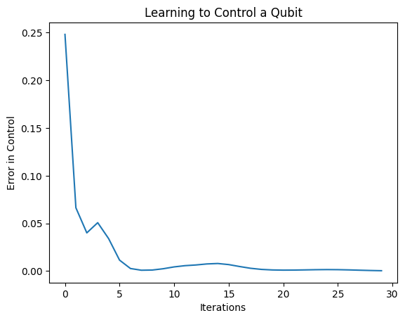
ฟังก์ชันการสูญเสียลดลงเหลือศูนย์

controller มีให้ในรูปแบบสแตนด์อโลน เรียกคอนโทรลเลอร์ และตรวจสอบการตอบสนองต่อสัญญาณคำสั่งแต่ละคำสั่ง จะต้องดำเนินการบางอย่างเพื่อเปรียบเทียบผลลัพธ์เหล่านี้กับเนื้อหาของ random_rotations อย่างถูกต้อง

controller.predict(np.array([0,1]))

array([[3.6335812 , 1.8470774 , 0.71675825],
       [5.3085413 , 0.08116499, 2.8337662 ]], dtype=float32)