
| | |  ดูแหล่งที่มาบน GitHub ดูแหล่งที่มาบน GitHub | |
import numpy as np
import matplotlib.pyplot as plt
import tensorflow.compat.v2 as tf
tf.enable_v2_behavior()

import tensorflow_probability as tfp
tfd = tfp.distributions
tfb = tfp.bijectors
[เชื่อม] (https://en.wikipedia.org/wiki/Copula_ (% probability_theory 29) เป็นวิธีการที่คลาสสิกสำหรับการจับภาพการพึ่งพาอาศัยกันระหว่างตัวแปรสุ่ม. เพิ่มเติมอย่างเป็นทางการที่เชื่อมเป็นหลายตัวแปรกระจาย \(C(U_1, U_2, ...., U_n)\) ดังกล่าวว่า marginalizing ให้ \(U_i \sim \text{Uniform}(0, 1)\)
Copulas นั้นน่าสนใจเพราะเราสามารถใช้พวกมันเพื่อสร้างการแจกแจงแบบหลายตัวแปรด้วยส่วนเพิ่มตามอำเภอใจ นี่คือสูตร:
- ใช้ เป็นส่วนประกอบสำคัญน่าจะเป็นเปลี่ยน ผลัดพล RV อย่างต่อเนื่อง \(X\) เข้าไปในเครื่องแบบหนึ่ง \(F_X(X)\)ที่ \(F_X\) เป็น CDF ของ \(X\)
- ได้รับการเชื่อม (พูด bivariate) \(C(U, V)\)เรามีที่ \(U\) และ \(V\) มีการกระจายร่อแร่เครื่องแบบ
- ตอนนี้ได้รับ RV ของเราที่น่าสนใจ \(X, Y\)สร้างใหม่กระจาย \(C'(X, Y) = C(F_X(X), F_Y(Y))\)มาร์จินสำหรับ \(X\) และ \(Y\) จะเป็นคนที่เราต้องการ
ระยะขอบไม่แปรผัน ดังนั้นจึงอาจวัดและ/หรือแบบจำลองได้ง่ายกว่า คอปูลาช่วยให้เริ่มต้นจากส่วนขอบ แต่ยังบรรลุความสัมพันธ์ตามอำเภอใจระหว่างมิติ
Gaussian Copula
เพื่อแสดงให้เห็นวิธีการสร้าง copulas ให้พิจารณากรณีของการจับการพึ่งพาตามสหสัมพันธ์แบบเกาส์เซียนพหุตัวแปร Gaussian เชื่อมเป็นหนึ่งที่ได้รับจาก \(C(u_1, u_2, ...u_n) = \Phi_\Sigma(\Phi^{-1}(u_1), \Phi^{-1}(u_2), ... \Phi^{-1}(u_n))\) ที่ \(\Phi_\Sigma\) หมายถึง CDF ของ MultivariateNormal ที่มีความแปรปรวน \(\Sigma\) และค่าเฉลี่ย 0 และ \(\Phi^{-1}\) เป็น CDF ผกผันสำหรับมาตรฐานปกติ
การใช้ CDF ผกผันปกติจะบิดเบือนมิติที่สม่ำเสมอเพื่อกระจายตามปกติ การใช้ CDF ของค่าปกติแบบพหุตัวแปรแล้วบีบการแจกแจงให้เป็นแบบเดียวกันเล็กน้อยและมีความสัมพันธ์แบบเกาส์เซียน
ดังนั้นสิ่งที่เราได้รับคือว่า Gaussian เชื่อมคือการกระจายมากกว่าหน่วย hypercube \([0, 1]^n\) กับมาร์จินเครื่องแบบ
กำหนดให้เป็นเช่นนั้นเสียนเชื่อมสามารถดำเนินการกับ tfd.TransformedDistribution และเหมาะสม Bijector นั่นก็คือเรามีการปรับเปลี่ยน MultivariateNormal, ผ่านการใช้งานของการกระจายปกติของผกผัน CDF ที่ดำเนินการโดย tfb.NormalCDF bijector
ด้านล่างเราใช้ Gaussian เชื่อมกับสมมติฐานการลดความซับซ้อน: ที่แปรปรวนจะแปรโดยปัจจัย Cholesky (ด้วยเหตุนี้ความแปรปรวนสำหรับ MultivariateNormalTriL ) (หนึ่งสามารถใช้อื่น ๆ tf.linalg.LinearOperators การเข้ารหัสสมมติฐานเมทริกซ์ฟรีที่แตกต่างกัน.)
class GaussianCopulaTriL(tfd.TransformedDistribution):
"""Takes a location, and lower triangular matrix for the Cholesky factor."""
def __init__(self, loc, scale_tril):
super(GaussianCopulaTriL, self).__init__(
distribution=tfd.MultivariateNormalTriL(
loc=loc,
scale_tril=scale_tril),
bijector=tfb.NormalCDF(),
validate_args=False,
name="GaussianCopulaTriLUniform")
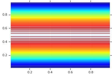
# Plot an example of this.
unit_interval = np.linspace(0.01, 0.99, num=200, dtype=np.float32)
x_grid, y_grid = np.meshgrid(unit_interval, unit_interval)
coordinates = np.concatenate(
[x_grid[..., np.newaxis],
y_grid[..., np.newaxis]], axis=-1)
pdf = GaussianCopulaTriL(
loc=[0., 0.],
scale_tril=[[1., 0.8], [0., 0.6]],
).prob(coordinates)
# Plot its density.
plt.contour(x_grid, y_grid, pdf, 100, cmap=plt.cm.jet);
อย่างไรก็ตาม พลังจากแบบจำลองดังกล่าวกำลังใช้ Probability Integral Transform เพื่อใช้ copula กับ RVs ที่กำหนดเอง ด้วยวิธีนี้ เราสามารถระบุ Marginals ตามอำเภอใจ และใช้ copula เพื่อต่อเข้าด้วยกัน
เราเริ่มต้นด้วยแบบจำลอง:
\[\begin{align*} X &\sim \text{Kumaraswamy}(a, b) \\ Y &\sim \text{Gumbel}(\mu, \beta) \end{align*}\]
และใช้เชื่อมที่จะได้รับ bivariate RV \(Z\)ซึ่งมีมาร์จิน Kumaraswamy และ กัมเบล
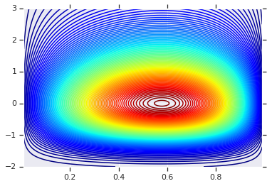
เราจะเริ่มต้นด้วยการวางแผนการกระจายผลิตภัณฑ์ที่สร้างโดย RV สองตัวนี้ นี่เป็นเพียงเพื่อใช้เป็นจุดเปรียบเทียบเมื่อเราใช้ Copula
a = 2.0
b = 2.0
gloc = 0.
gscale = 1.

x = tfd.Kumaraswamy(a, b)
y = tfd.Gumbel(loc=gloc, scale=gscale)

# Plot the distributions, assuming independence
x_axis_interval = np.linspace(0.01, 0.99, num=200, dtype=np.float32)
y_axis_interval = np.linspace(-2., 3., num=200, dtype=np.float32)
x_grid, y_grid = np.meshgrid(x_axis_interval, y_axis_interval)

pdf = x.prob(x_grid) * y.prob(y_grid)

# Plot its density

plt.contour(x_grid, y_grid, pdf, 100, cmap=plt.cm.jet);
การกระจายร่วมกับขอบต่างกัน
ตอนนี้เราใช้คอปูลาเกาส์เซียนเพื่อรวมการแจกแจงเข้าด้วยกัน และพลอตมัน อีกครั้งเครื่องมือของทางเลือกของเราคือการ TransformedDistribution ใช้ที่เหมาะสม Bijector ที่จะได้รับมาร์จินที่เลือก
โดยเฉพาะเราใช้ Blockwise bijector ซึ่งใช้ bijectors แตกต่างกันในส่วนต่าง ๆ ของเวกเตอร์ (ซึ่งยังคงเป็นการเปลี่ยนแปลง bijective)
ตอนนี้เราสามารถกำหนด Copula ที่เราต้องการได้ จากรายชื่อเป้าหมายเป้าหมาย (เข้ารหัสเป็น bijectors) เราสามารถสร้างการกระจายใหม่ที่ใช้ copula และมีระยะขอบที่ระบุได้อย่างง่ายดาย
class WarpedGaussianCopula(tfd.TransformedDistribution):
  """Application of a Gaussian Copula on a list of target marginals.

  This implements an application of a Gaussian Copula. Given [x_0, ... x_n]
  which are distributed marginally (with CDF) [F_0, ... F_n],
  `GaussianCopula` represents an application of the Copula, such that the
  resulting multivariate distribution has the above specified marginals.

  The marginals are specified by `marginal_bijectors`: These are
  bijectors whose `inverse` encodes the CDF and `forward` the inverse CDF.

  block_sizes is a 1-D Tensor to determine splits for `marginal_bijectors`
  length should be same as length of `marginal_bijectors`.
  See tfb.Blockwise for details
  """
  def __init__(self, loc, scale_tril, marginal_bijectors, block_sizes=None):
    super(WarpedGaussianCopula, self).__init__(
        distribution=GaussianCopulaTriL(loc=loc, scale_tril=scale_tril),
        bijector=tfb.Blockwise(bijectors=marginal_bijectors,
                               block_sizes=block_sizes),
        validate_args=False,
        name="GaussianCopula")
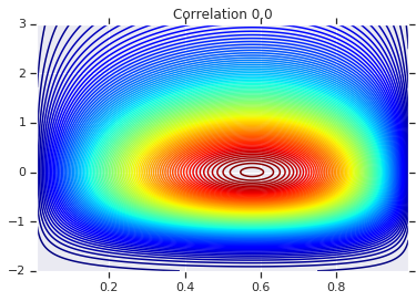
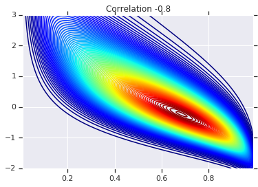
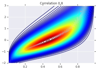
สุดท้ายนี้ เรามาลองใช้ Gaussian Copula กันดีกว่า เราจะใช้ Cholesky ของ \(\begin{bmatrix}1 & 0\\\rho & \sqrt{(1-\rho^2)}\end{bmatrix}\)ซึ่งจะสอดคล้องกับความแปรปรวนที่ 1 และความสัมพันธ์ \(\rho\) สำหรับหลายตัวแปรปกติ
เราจะพิจารณาบางกรณี:
# Create our coordinates:
coordinates = np.concatenate(
    [x_grid[..., np.newaxis], y_grid[..., np.newaxis]], -1)


def create_gaussian_copula(correlation):
  # Use Gaussian Copula to add dependence.
  return WarpedGaussianCopula(
      loc=[0.,  0.],
      scale_tril=[[1., 0.], [correlation, tf.sqrt(1. - correlation ** 2)]],
      # These encode the marginals we want. In this case we want X_0 has
      # Kumaraswamy marginal, and X_1 has Gumbel marginal.

      marginal_bijectors=[
          tfb.Invert(tfb.KumaraswamyCDF(a, b)),
          tfb.Invert(tfb.GumbelCDF(loc=0., scale=1.))])


# Note that the zero case will correspond to independent marginals!
correlations = [0., -0.8, 0.8]
copulas = []
probs = []
for correlation in correlations:
  copula = create_gaussian_copula(correlation)
  copulas.append(copula)
  probs.append(copula.prob(coordinates))


# Plot it's density

for correlation, copula_prob in zip(correlations, probs):
  plt.figure()
  plt.contour(x_grid, y_grid, copula_prob, 100, cmap=plt.cm.jet)
  plt.title('Correlation {}'.format(correlation))
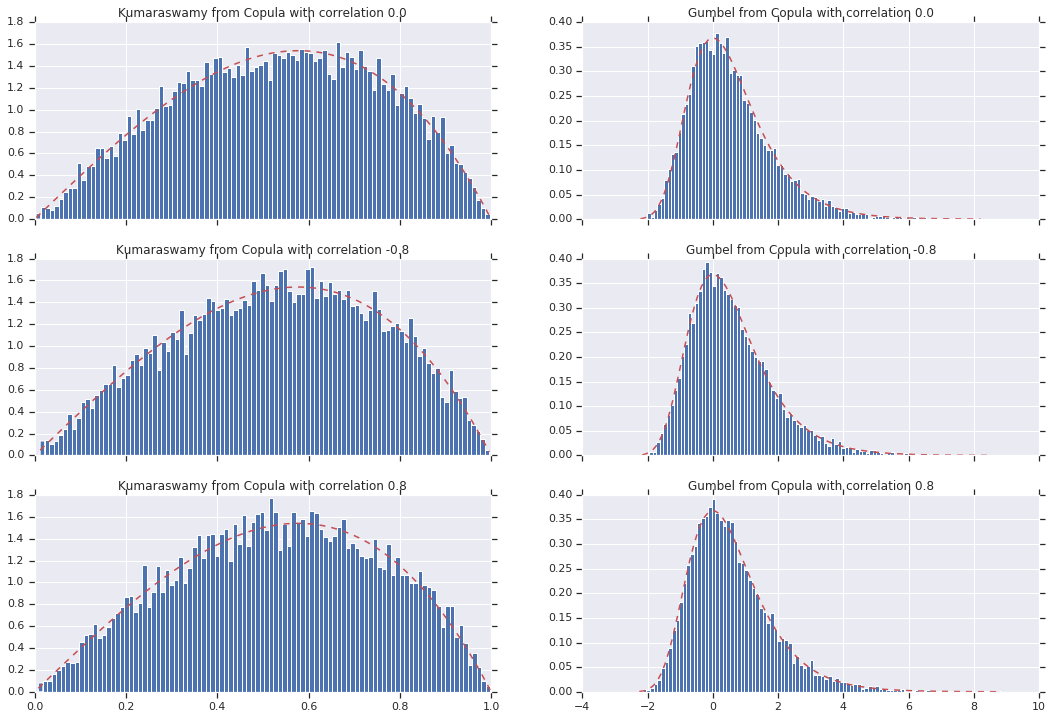
สุดท้าย มาตรวจสอบกันว่าเราได้ส่วนเพิ่มที่เราต้องการจริง ๆ แล้ว
def kumaraswamy_pdf(x):
    return tfd.Kumaraswamy(a, b).prob(np.float32(x))

def gumbel_pdf(x):
    return tfd.Gumbel(gloc, gscale).prob(np.float32(x))


copula_samples = []
for copula in copulas:
  copula_samples.append(copula.sample(10000))

plot_rows = len(correlations)
plot_cols = 2  # for 2  densities [kumarswamy, gumbel]
fig, axes = plt.subplots(plot_rows, plot_cols, sharex='col', figsize=(18,12))

# Let's marginalize out on each, and plot the samples.

for i, (correlation, copula_sample) in enumerate(zip(correlations, copula_samples)):
  k = copula_sample[..., 0].numpy()
  g = copula_sample[..., 1].numpy()


  _, bins, _ = axes[i, 0].hist(k, bins=100, density=True)
  axes[i, 0].plot(bins, kumaraswamy_pdf(bins), 'r--')
  axes[i, 0].set_title('Kumaraswamy from Copula with correlation {}'.format(correlation))

  _, bins, _ = axes[i, 1].hist(g, bins=100, density=True)
  axes[i, 1].plot(bins, gumbel_pdf(bins), 'r--')
  axes[i, 1].set_title('Gumbel from Copula with correlation {}'.format(correlation))
บทสรุป
และเราไปกันเลย! เราได้แสดงให้เห็นว่าเราสามารถสร้างแบบเกาส์ Copulas ใช้ Bijector API
โดยทั่วไปการเขียน bijectors ใช้ Bijector API และเขียนพวกเขาด้วยการจัดจำหน่ายที่สามารถสร้างครอบครัวที่อุดมไปด้วยการกระจายสำหรับการสร้างแบบจำลองที่มีความยืดหยุ่น