
| | |  ดูแหล่งที่มาบน GitHub ดูแหล่งที่มาบน GitHub | |
ใน colab นี้ เราจะสำรวจกระบวนการถดถอยแบบเกาส์เซียนโดยใช้ TensorFlow และความน่าจะเป็นของ TensorFlow เราสร้างข้อสังเกตที่มีเสียงดังจากฟังก์ชันที่รู้จักและปรับโมเดล GP ให้เข้ากับข้อมูลเหล่านั้น จากนั้นเราสุ่มตัวอย่างจากส่วนหลังของ GP และพล็อตค่าฟังก์ชันตัวอย่างบนกริดในโดเมน
พื้นหลัง
ให้ \(\mathcal{X}\) เป็นชุดใด ๆ Gaussian กระบวนการ (GP) เป็นคอลเลกชันของตัวแปรสุ่มดัชนีโดย \(\mathcal{X}\) เช่นว่าถ้า\(\{X_1, \ldots, X_n\} \subset \mathcal{X}\) ใดเซต จำกัด ความหนาแน่นร่อแร่\(p(X_1 = x_1, \ldots, X_n = x_n)\) เป็นหลายตัวแปรแบบเกาส์ การแจกแจงแบบเกาส์เซียนใดๆ จะถูกระบุโดยสมบูรณ์โดยโมเมนต์ศูนย์กลางที่หนึ่งและที่สอง (ค่าเฉลี่ยและความแปรปรวนร่วม) และค่า GP ก็ไม่มีข้อยกเว้น เราสามารถระบุ GP สมบูรณ์ในแง่ของค่าเฉลี่ยการทำงานของ \(\mu : \mathcal{X} \to \mathbb{R}\) และฟังก์ชั่นความแปรปรวน\(k : \mathcal{X} \times \mathcal{X} \to \mathbb{R}\)พลังการแสดงออกส่วนใหญ่ของ GP ถูกห่อหุ้มไว้ในการเลือกฟังก์ชันความแปรปรวนร่วม ด้วยเหตุผลต่างๆฟังก์ชั่นความแปรปรวนยังจะเรียกว่าเป็นฟังก์ชั่นเคอร์เนล มันเป็นสิ่งจำเป็นเท่านั้นที่จะสมมาตรและบวกที่ชัดเจน (ดู Ch. 4 ของรัสมุสและวิลเลียมส์ ) ด้านล่างเราใช้เคอร์เนลความแปรปรวนร่วมกำลังสอง รูปแบบของมันคือ
\[ k(x, x') := \sigma^2 \exp \left( \frac{\|x - x'\|^2}{\lambda^2} \right) \]
ที่ \(\sigma^2\) เรียกว่า 'กว้าง' และ \(\lambda\) ขนาดความยาว พารามิเตอร์เคอร์เนลสามารถเลือกได้ผ่านขั้นตอนการเพิ่มประสิทธิภาพความน่าจะเป็นสูงสุด
ตัวอย่างเต็มรูปแบบจาก GP ประกอบด้วยฟังก์ชั่นแบบ real-มูลค่ามากกว่าทั้งพื้นที่\(\mathcal{X}\) และเป็นในทางปฏิบัติทำไม่ได้ที่จะตระหนักถึง; มักจะเลือกชุดของจุดที่สังเกตตัวอย่างและดึงค่าฟังก์ชันที่จุดเหล่านี้ ทำได้โดยการสุ่มตัวอย่างจาก Gaussian หลายตัวแปรที่เหมาะสม (จำกัดมิติ)
โปรดทราบว่า ตามคำจำกัดความข้างต้น การแจกแจงหลายตัวแปรแบบหลายตัวแปรที่มีขอบเขตจำกัดใดๆ ก็เป็นกระบวนการแบบเกาส์เซียนเช่นกัน โดยปกติเมื่อหนึ่งหมายถึง GP มันเป็นนัยที่ SET Index เป็นบาง \(\mathbb{R}^n\)และแน่นอนเราจะทำให้สมมติฐานนี้ที่นี่
การประยุกต์ใช้กระบวนการเกาส์เซียนทั่วไปในการเรียนรู้ของเครื่องคือการถดถอยกระบวนการเกาส์เซียน แนวคิดก็คือว่าเราต้องการที่จะประเมินฟังก์ชั่นที่ไม่รู้จักให้สังเกตที่มีเสียงดัง \(\{y_1, \ldots, y_N\}\) ของฟังก์ชั่นที่จำนวน จำกัด ของจุด \(\{x_1, \ldots x_N\}.\) เราจินตนาการกระบวนการกำเนิด
\[ \begin{align} f \sim \: & \textsf{GaussianProcess}\left( \text{mean_fn}=\mu(x), \text{covariance_fn}=k(x, x')\right) \\ y_i \sim \: & \textsf{Normal}\left( \text{loc}=f(x_i), \text{scale}=\sigma\right), i = 1, \ldots, N \end{align} \]
ดังที่กล่าวไว้ข้างต้น ฟังก์ชันสุ่มตัวอย่างไม่สามารถคำนวณได้ เนื่องจากเราต้องการค่าของมันที่จุดจำนวนอนันต์ แทนที่จะพิจารณาตัวอย่างที่มีขอบเขตจาก Gaussian หลายตัวแปร
\[ \begin{gather} \begin{bmatrix} f(x_1) \\ \vdots \\ f(x_N) \end{bmatrix} \sim \textsf{MultivariateNormal} \left( \: \text{loc}= \begin{bmatrix} \mu(x_1) \\ \vdots \\ \mu(x_N) \end{bmatrix} \:,\: \text{scale}= \begin{bmatrix} k(x_1, x_1) & \cdots & k(x_1, x_N) \\ \vdots & \ddots & \vdots \\ k(x_N, x_1) & \cdots & k(x_N, x_N) \\ \end{bmatrix}^{1/2} \: \right) \end{gather} \\ y_i \sim \textsf{Normal} \left( \text{loc}=f(x_i), \text{scale}=\sigma \right) \]
หมายเหตุสัญลักษณ์ \(\frac{1}{2}\) บนเมทริกซ์ความแปรปรวนร่วม: นี้หมายถึงการสลายตัว Cholesky การคำนวณ Cholesky เป็นสิ่งจำเป็นเนื่องจาก MVN เป็นการกระจายตระกูลตามตำแหน่ง แต่น่าเสียดายที่การสลายตัว Cholesky แพงคอมพิวเตอร์, การ \(O(N^3)\) เวลาและ \(O(N^2)\) พื้นที่ วรรณคดี GP ส่วนใหญ่มุ่งเน้นไปที่การจัดการกับเลขชี้กำลังเล็กน้อยที่ดูเหมือนไม่มีพิษภัยนี้
เป็นเรื่องปกติที่จะให้ฟังก์ชันค่าเฉลี่ยก่อนหน้าเป็นค่าคงที่ ซึ่งมักจะเป็นศูนย์ นอกจากนี้ อนุสัญญาสัญกรณ์บางอย่างก็สะดวกเช่นกัน หนึ่งมักจะเขียน \(\mathbf{f}\) สำหรับเวกเตอร์ จำกัด ของค่าฟังก์ชั่นตัวอย่าง จำนวนข้อความที่น่าสนใจที่จะใช้สำหรับเมทริกซ์ความแปรปรวนที่เกิดจากการประยุกต์ใช้ \(k\) เพื่อคู่ของปัจจัยการผลิต ดังต่อไปนี้ (Quiñonero-Candela 2005) เราทราบว่าองค์ประกอบของเมทริกซ์ที่มี covariances ของค่าฟังก์ชั่นที่จุดป้อนข้อมูลโดยเฉพาะอย่างยิ่ง ดังนั้นเราสามารถแสดงเมทริกซ์ความแปรปรวนเป็น \(K_{AB}\)ที่ \(A\) และ \(B\) เป็นตัวชี้วัดบางส่วนของคอลเลกชันของค่าฟังก์ชั่นพร้อมรับมิติเมทริกซ์
ตัวอย่างเช่นกำหนดข้อมูลที่สังเกต \((\mathbf{x}, \mathbf{y})\) มีนัยค่าฟังก์ชั่นที่แฝง \(\mathbf{f}\)เราสามารถเขียน
\[ K_{\mathbf{f},\mathbf{f} } = \begin{bmatrix} k(x_1, x_1) & \cdots & k(x_1, x_N) \\ \vdots & \ddots & \vdots \\ k(x_N, x_1) & \cdots & k(x_N, x_N) \\ \end{bmatrix} \]
ในทำนองเดียวกัน เราสามารถผสมชุดอินพุตได้ เช่น in
\[ K_{\mathbf{f},*} = \begin{bmatrix} k(x_1, x^*_1) & \cdots & k(x_1, x^*_T) \\ \vdots & \ddots & \vdots \\ k(x_N, x^*_1) & \cdots & k(x_N, x^*_T) \\ \end{bmatrix} \]
ที่เราคิดว่ามี \(N\) ปัจจัยการผลิตการฝึกอบรมและ \(T\) ปัจจัยการผลิตการทดสอบ กระบวนการกำเนิดข้างต้นอาจเขียนกระชับเป็น
\[ \begin{align} \mathbf{f} \sim \: & \textsf{MultivariateNormal} \left( \text{loc}=\mathbf{0}, \text{scale}=K_{\mathbf{f},\mathbf{f} }^{1/2} \right) \\ y_i \sim \: & \textsf{Normal} \left( \text{loc}=f_i, \text{scale}=\sigma \right), i = 1, \ldots, N \end{align} \]
การดำเนินการสุ่มตัวอย่างในบรรทัดแรกมีผลเป็นชุด จำกัด ของ \(N\) ค่าฟังก์ชั่นจากหลายตัวแปรแบบเกาส์ - ไม่ฟังก์ชั่นทั้งหมดเป็นในข้างต้น GP วาดสัญกรณ์ บรรทัดที่สองอธิบายถึงคอลเลกชันของ \(N\) ดึงออกมาจาก univariate Gaussians ศูนย์กลางที่ค่าฟังก์ชั่นต่าง ๆ ที่มีสัญญาณรบกวนการสังเกตคง \(\sigma^2\)
ด้วยแบบจำลองกำเนิดข้างต้น เราสามารถดำเนินการพิจารณาปัญหาการอนุมานภายหลังได้ สิ่งนี้ให้ผลการแจกแจงภายหลังเหนือค่าฟังก์ชันที่จุดทดสอบชุดใหม่ ซึ่งกำหนดเงื่อนไขตามข้อมูลรบกวนที่สังเกตได้จากกระบวนการด้านบน
ด้วยสัญกรณ์ดังกล่าวข้างต้นในสถานที่ที่เราสามารถเขียนดานการกระจายการทำนายหลังมากกว่าในอนาคต (มีเสียงดัง) สังเกตเงื่อนไขในปัจจัยการผลิตและข้อมูลการฝึกอบรมที่เกี่ยวข้องดังต่อไปนี้ (สำหรับรายละเอียดเพิ่มเติมโปรดดูที่§2.2ของ รัสมุสและวิลเลียมส์ )
\[ \mathbf{y}^* \mid \mathbf{x}^*, \mathbf{x}, \mathbf{y} \sim \textsf{Normal} \left( \text{loc}=\mathbf{\mu}^*, \text{scale}=(\Sigma^*)^{1/2} \right), \]
ที่ไหน
\[ \mathbf{\mu}^* = K_{*,\mathbf{f} }\left(K_{\mathbf{f},\mathbf{f} } + \sigma^2 I \right)^{-1} \mathbf{y} \]
และ
\[ \Sigma^* = K_{*,*} - K_{*,\mathbf{f} } \left(K_{\mathbf{f},\mathbf{f} } + \sigma^2 I \right)^{-1} K_{\mathbf{f},*} \]
นำเข้า
import time

import numpy as np
import matplotlib.pyplot as plt
import tensorflow.compat.v2 as tf
import tensorflow_probability as tfp
tfb = tfp.bijectors
tfd = tfp.distributions
tfk = tfp.math.psd_kernels
tf.enable_v2_behavior()

from mpl_toolkits.mplot3d import Axes3D
%pylab inline
# Configure plot defaults
plt.rcParams['axes.facecolor'] = 'white'
plt.rcParams['grid.color'] = '#666666'
%config InlineBackend.figure_format = 'png'
Populating the interactive namespace from numpy and matplotlib
ตัวอย่าง: การถดถอย GP ที่แน่นอนบนข้อมูลไซนัสที่มีเสียงดัง
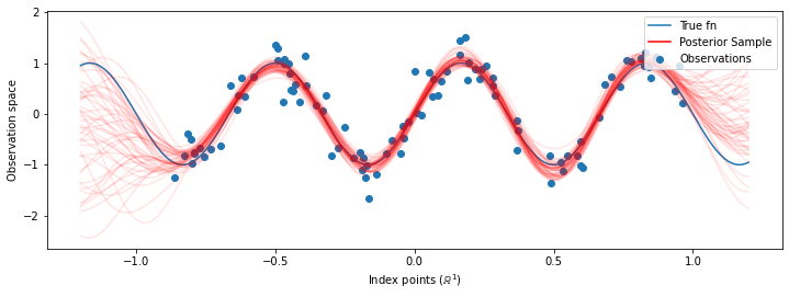
ที่นี่ เราสร้างข้อมูลการฝึกจากไซนูซอยด์ที่มีเสียงดัง จากนั้นสุ่มตัวอย่างเส้นโค้งจำนวนหนึ่งจากส่วนหลังของแบบจำลองการถดถอย GP เราใช้ อดัม เพื่อเพิ่มประสิทธิภาพ hyperparameters เคอร์เนล (เราลดโอกาสในการเข้าสู่ระบบในเชิงลบของข้อมูลภายใต้ก่อนหน้านี้) เราวาดเส้นโค้งการฝึก ตามด้วยฟังก์ชันจริงและตัวอย่างหลัง
def sinusoid(x):
  return np.sin(3 * np.pi * x[..., 0])

def generate_1d_data(num_training_points, observation_noise_variance):
  """Generate noisy sinusoidal observations at a random set of points.

  Returns:
     observation_index_points, observations
  """
  index_points_ = np.random.uniform(-1., 1., (num_training_points, 1))
  index_points_ = index_points_.astype(np.float64)
  # y = f(x) + noise
  observations_ = (sinusoid(index_points_) +
                   np.random.normal(loc=0,
                                    scale=np.sqrt(observation_noise_variance),
                                    size=(num_training_points)))
  return index_points_, observations_
# Generate training data with a known noise level (we'll later try to recover
# this value from the data).
NUM_TRAINING_POINTS = 100
observation_index_points_, observations_ = generate_1d_data(
    num_training_points=NUM_TRAINING_POINTS,
    observation_noise_variance=.1)
เราจะใส่ไพรเออร์ใน hyperparameters เคอร์เนลและเขียนร่วมกันจำหน่ายของ hyperparameters และสังเกตข้อมูลโดยใช้ tfd.JointDistributionNamed
def build_gp(amplitude, length_scale, observation_noise_variance):
  """Defines the conditional dist. of GP outputs, given kernel parameters."""

  # Create the covariance kernel, which will be shared between the prior (which we
  # use for maximum likelihood training) and the posterior (which we use for
  # posterior predictive sampling)
  kernel = tfk.ExponentiatedQuadratic(amplitude, length_scale)

  # Create the GP prior distribution, which we will use to train the model
  # parameters.
  return tfd.GaussianProcess(
      kernel=kernel,
      index_points=observation_index_points_,
      observation_noise_variance=observation_noise_variance)

gp_joint_model = tfd.JointDistributionNamed({
    'amplitude': tfd.LogNormal(loc=0., scale=np.float64(1.)),
    'length_scale': tfd.LogNormal(loc=0., scale=np.float64(1.)),
    'observation_noise_variance': tfd.LogNormal(loc=0., scale=np.float64(1.)),
    'observations': build_gp,
})
เราสามารถตรวจสอบการใช้งานของเราอย่างมีสติโดยตรวจสอบว่าเราสามารถสุ่มตัวอย่างจากก่อนหน้านี้ และคำนวณความหนาแน่นของบันทึกของกลุ่มตัวอย่าง
x = gp_joint_model.sample()
lp = gp_joint_model.log_prob(x)

print("sampled {}".format(x))
print("log_prob of sample: {}".format(lp))
sampled {'observation_noise_variance': <tf.Tensor: shape=(), dtype=float64, numpy=2.067952217184325>, 'length_scale': <tf.Tensor: shape=(), dtype=float64, numpy=1.154435715487831>, 'amplitude': <tf.Tensor: shape=(), dtype=float64, numpy=5.383850737703549>, 'observations': <tf.Tensor: shape=(100,), dtype=float64, numpy=
array([-2.37070577, -2.05363838, -0.95152824,  3.73509388, -0.2912646 ,
        0.46112342, -1.98018513, -2.10295857, -1.33589756, -2.23027226,
       -2.25081374, -0.89450835, -2.54196452,  1.46621647,  2.32016193,
        5.82399989,  2.27241034, -0.67523432, -1.89150197, -1.39834474,
       -2.33954116,  0.7785609 , -1.42763627, -0.57389025, -0.18226098,
       -3.45098732,  0.27986652, -3.64532398, -1.28635204, -2.42362875,
        0.01107288, -2.53222176, -2.0886136 , -5.54047694, -2.18389607,
       -1.11665628, -3.07161217, -2.06070336, -0.84464262,  1.29238438,
       -0.64973999, -2.63805504, -3.93317576,  0.65546645,  2.24721181,
       -0.73403676,  5.31628298, -1.2208384 ,  4.77782252, -1.42978168,
       -3.3089274 ,  3.25370494,  3.02117591, -1.54862932, -1.07360811,
        1.2004856 , -4.3017773 , -4.95787789, -1.95245901, -2.15960839,
       -3.78592731, -1.74096185,  3.54891595,  0.56294143,  1.15288455,
       -0.77323696,  2.34430694, -1.05302007, -0.7514684 , -0.98321063,
       -3.01300144, -3.00033274,  0.44200837,  0.45060886, -1.84497318,
       -1.89616746, -2.15647664, -2.65672581, -3.65493379,  1.70923375,
       -3.88695218, -0.05151283,  4.51906677, -2.28117003,  3.03032793,
       -1.47713194, -0.35625273,  3.73501587, -2.09328047, -0.60665614,
       -0.78177188, -0.67298545,  2.97436033, -0.29407932,  2.98482427,
       -1.54951178,  2.79206821,  4.2225733 ,  2.56265198,  2.80373284])>}
log_prob of sample: -194.96442183797524
ตอนนี้ มาเพิ่มประสิทธิภาพเพื่อค้นหาค่าพารามิเตอร์ที่มีความน่าจะเป็นหลังสูงสุด เราจะกำหนดตัวแปรสำหรับแต่ละพารามิเตอร์ และจำกัดค่าให้เป็นค่าบวก
# Create the trainable model parameters, which we'll subsequently optimize.
# Note that we constrain them to be strictly positive.

constrain_positive = tfb.Shift(np.finfo(np.float64).tiny)(tfb.Exp())

amplitude_var = tfp.util.TransformedVariable(
    initial_value=1.,
    bijector=constrain_positive,
    name='amplitude',
    dtype=np.float64)

length_scale_var = tfp.util.TransformedVariable(
    initial_value=1.,
    bijector=constrain_positive,
    name='length_scale',
    dtype=np.float64)

observation_noise_variance_var = tfp.util.TransformedVariable(
    initial_value=1.,
    bijector=constrain_positive,
    name='observation_noise_variance_var',
    dtype=np.float64)

trainable_variables = [v.trainable_variables[0] for v in
                       [amplitude_var,
                       length_scale_var,
                       observation_noise_variance_var]]
ไปอยู่ในสภาพแบบกับข้อมูลที่สังเกตของเราเราจะกำหนด target_log_prob ฟังก์ชั่นซึ่งจะนำ (ยังคงที่จะอนุมาน) เคอร์เนล hyperparameters
def target_log_prob(amplitude, length_scale, observation_noise_variance):
  return gp_joint_model.log_prob({
      'amplitude': amplitude,
      'length_scale': length_scale,
      'observation_noise_variance': observation_noise_variance,
      'observations': observations_
  })
# Now we optimize the model parameters.
num_iters = 1000
optimizer = tf.optimizers.Adam(learning_rate=.01)

# Use `tf.function` to trace the loss for more efficient evaluation.
@tf.function(autograph=False, jit_compile=False)
def train_model():
  with tf.GradientTape() as tape:
    loss = -target_log_prob(amplitude_var, length_scale_var,
                            observation_noise_variance_var)
  grads = tape.gradient(loss, trainable_variables)
  optimizer.apply_gradients(zip(grads, trainable_variables))
  return loss

# Store the likelihood values during training, so we can plot the progress
lls_ = np.zeros(num_iters, np.float64)
for i in range(num_iters):
  loss = train_model()
  lls_[i] = loss

print('Trained parameters:')
print('amplitude: {}'.format(amplitude_var._value().numpy()))
print('length_scale: {}'.format(length_scale_var._value().numpy()))
print('observation_noise_variance: {}'.format(observation_noise_variance_var._value().numpy()))
Trained parameters:
amplitude: 0.9176153445125278
length_scale: 0.18444082442910079
observation_noise_variance: 0.0880273312850989
# Plot the loss evolution
plt.figure(figsize=(12, 4))
plt.plot(lls_)
plt.xlabel("Training iteration")
plt.ylabel("Log marginal likelihood")
plt.show()

# Having trained the model, we'd like to sample from the posterior conditioned
# on observations. We'd like the samples to be at points other than the training
# inputs.
predictive_index_points_ = np.linspace(-1.2, 1.2, 200, dtype=np.float64)
# Reshape to [200, 1] -- 1 is the dimensionality of the feature space.
predictive_index_points_ = predictive_index_points_[..., np.newaxis]

optimized_kernel = tfk.ExponentiatedQuadratic(amplitude_var, length_scale_var)
gprm = tfd.GaussianProcessRegressionModel(
    kernel=optimized_kernel,
    index_points=predictive_index_points_,
    observation_index_points=observation_index_points_,
    observations=observations_,
    observation_noise_variance=observation_noise_variance_var,
    predictive_noise_variance=0.)

# Create op to draw  50 independent samples, each of which is a *joint* draw
# from the posterior at the predictive_index_points_. Since we have 200 input
# locations as defined above, this posterior distribution over corresponding
# function values is a 200-dimensional multivariate Gaussian distribution!
num_samples = 50
samples = gprm.sample(num_samples)
# Plot the true function, observations, and posterior samples.
plt.figure(figsize=(12, 4))
plt.plot(predictive_index_points_, sinusoid(predictive_index_points_),
         label='True fn')
plt.scatter(observation_index_points_[:, 0], observations_,
            label='Observations')
for i in range(num_samples):
  plt.plot(predictive_index_points_, samples[i, :], c='r', alpha=.1,
           label='Posterior Sample' if i == 0 else None)
leg = plt.legend(loc='upper right')
for lh in leg.legendHandles:
    lh.set_alpha(1)
plt.xlabel(r"Index points ($\mathbb{R}^1$)")
plt.ylabel("Observation space")
plt.show()
การเพิ่มขอบของไฮเปอร์พารามิเตอร์ด้วย HMC
แทนที่จะเพิ่มประสิทธิภาพไฮเปอร์พารามิเตอร์ ให้ลองรวมเข้ากับ Hamiltonian Monte Carlo ก่อนอื่นเราจะกำหนดและเรียกใช้ตัวอย่างเพื่อดึงโดยประมาณจากการแจกแจงภายหลังเหนือเคอร์เนลไฮเปอร์พารามิเตอร์ตามข้อสังเกต
num_results = 100
num_burnin_steps = 50

sampler = tfp.mcmc.TransformedTransitionKernel(
    tfp.mcmc.NoUTurnSampler(
        target_log_prob_fn=target_log_prob,
        step_size=tf.cast(0.1, tf.float64)),
    bijector=[constrain_positive, constrain_positive, constrain_positive])

adaptive_sampler = tfp.mcmc.DualAveragingStepSizeAdaptation(
    inner_kernel=sampler,
    num_adaptation_steps=int(0.8 * num_burnin_steps),
    target_accept_prob=tf.cast(0.75, tf.float64))

initial_state = [tf.cast(x, tf.float64) for x in [1., 1., 1.]]
# Speed up sampling by tracing with `tf.function`.
@tf.function(autograph=False, jit_compile=False)
def do_sampling():
  return tfp.mcmc.sample_chain(
      kernel=adaptive_sampler,
      current_state=initial_state,
      num_results=num_results,
      num_burnin_steps=num_burnin_steps,
      trace_fn=lambda current_state, kernel_results: kernel_results)

t0 = time.time()
samples, kernel_results = do_sampling()
t1 = time.time()
print("Inference ran in {:.2f}s.".format(t1-t0))
Inference ran in 9.00s.
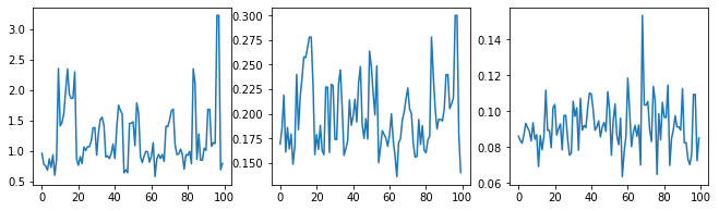
มาตรวจสุขภาพจิตกัน-ตรวจสอบแซมเพลอร์โดยตรวจติดตามไฮเปอร์พารามิเตอร์
(amplitude_samples,
 length_scale_samples,
 observation_noise_variance_samples) = samples

f = plt.figure(figsize=[15, 3])
for i, s in enumerate(samples):
  ax = f.add_subplot(1, len(samples) + 1, i + 1)
  ax.plot(s)
ตอนนี้แทนการสร้าง GP เดียวกับ hyperparameters ที่ดีที่สุดที่เราสร้างการกระจายการทำนายหลังเป็นส่วนผสมของจีพีเอสแต่ละที่กำหนดโดยตัวอย่างจากการกระจายหลังมากกว่า hyperparameters สิ่งนี้จะรวมเข้ากับพารามิเตอร์หลังโดยประมาณผ่านการสุ่มตัวอย่างมอนติคาร์โลเพื่อคำนวณการแจกแจงแบบคาดการณ์ส่วนเพิ่มในตำแหน่งที่ไม่มีใครสังเกต
# The sampled hyperparams have a leading batch dimension, `[num_results, ...]`,
# so they construct a *batch* of kernels.
batch_of_posterior_kernels = tfk.ExponentiatedQuadratic(
    amplitude_samples, length_scale_samples)

# The batch of kernels creates a batch of GP predictive models, one for each
# posterior sample.
batch_gprm = tfd.GaussianProcessRegressionModel(
    kernel=batch_of_posterior_kernels,
    index_points=predictive_index_points_,
    observation_index_points=observation_index_points_,
    observations=observations_,
    observation_noise_variance=observation_noise_variance_samples,
    predictive_noise_variance=0.)

# To construct the marginal predictive distribution, we average with uniform
# weight over the posterior samples.
predictive_gprm = tfd.MixtureSameFamily(
    mixture_distribution=tfd.Categorical(logits=tf.zeros([num_results])),
    components_distribution=batch_gprm)

num_samples = 50
samples = predictive_gprm.sample(num_samples)
# Plot the true function, observations, and posterior samples.
plt.figure(figsize=(12, 4))
plt.plot(predictive_index_points_, sinusoid(predictive_index_points_),
         label='True fn')
plt.scatter(observation_index_points_[:, 0], observations_,
            label='Observations')
for i in range(num_samples):
  plt.plot(predictive_index_points_, samples[i, :], c='r', alpha=.1,
           label='Posterior Sample' if i == 0 else None)
leg = plt.legend(loc='upper right')
for lh in leg.legendHandles:
    lh.set_alpha(1)
plt.xlabel(r"Index points ($\mathbb{R}^1$)")
plt.ylabel("Observation space")
plt.show()
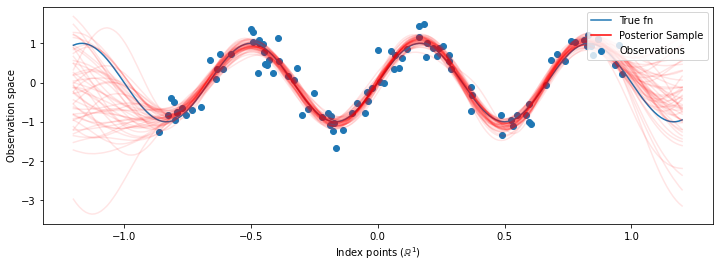
แม้ว่าความแตกต่างจะละเอียดในกรณีนี้ แต่โดยทั่วไป เราคาดว่าการแจกแจงแบบคาดการณ์ภายหลังจะสรุปได้ดีกว่า (ให้โอกาสที่สูงกว่าที่จะระงับข้อมูล) มากกว่าแค่การใช้พารามิเตอร์ที่น่าจะเป็นไปได้มากที่สุดดังที่เราทำข้างต้น