
| | |  ดูแหล่งที่มาบน GitHub ดูแหล่งที่มาบน GitHub | |
TensorFlow ความน่าจะเป็น (TFP) เป็นห้องสมุดสำหรับเหตุผลน่าจะเป็นและการวิเคราะห์ทางสถิติที่ตอนนี้ยังทำงานบน JAX ! สำหรับผู้ที่ไม่คุ้นเคย JAX เป็นไลบรารีสำหรับการประมวลผลเชิงตัวเลขแบบเร่งความเร็วโดยอิงจากการแปลงฟังก์ชันที่เขียนได้
TFP บน JAX รองรับการทำงานที่มีประโยชน์มากที่สุดของ TFP ปกติ ในขณะที่ยังคงรักษา abstractions และ API ที่ผู้ใช้ TFP จำนวนมากรู้สึกสบายใจ
ติดตั้ง
TFP ใน JAX ไม่ขึ้นอยู่กับ TensorFlow; ถอนการติดตั้ง TensorFlow จาก Colab นี้โดยสิ้นเชิง
pip uninstall tensorflow -y -q
เราสามารถติดตั้ง TFP บน JAX ด้วย TFP รุ่นล่าสุดทุกคืน
pip install -Uq tfp-nightly[jax] > /dev/null
มานำเข้าไลบรารี Python ที่มีประโยชน์กันเถอะ
import matplotlib.pyplot as plt
import numpy as np
import seaborn as sns
from sklearn import datasets
sns.set(style='white')
/usr/local/lib/python3.6/dist-packages/statsmodels/tools/_testing.py:19: FutureWarning: pandas.util.testing is deprecated. Use the functions in the public API at pandas.testing instead.
  import pandas.util.testing as tm
มานำเข้าฟังก์ชัน JAX พื้นฐานกันด้วย
import jax.numpy as jnp
from jax import grad
from jax import jit
from jax import random
from jax import value_and_grad
from jax import vmap
การนำเข้า TFP บน JAX
ที่จะใช้ใน TFP JAX เพียงแค่นำเข้า jax "สารตั้งต้น" และใช้เป็นคุณมักจะ tfp :
from tensorflow_probability.substrates import jax as tfp
tfd = tfp.distributions
tfb = tfp.bijectors
tfpk = tfp.math.psd_kernels
การสาธิต: การถดถอยโลจิสติกแบบเบย์
เพื่อแสดงให้เห็นว่าเราสามารถทำอะไรกับแบ็กเอนด์ JAX ได้บ้าง เราจะนำการถดถอยโลจิสติกแบบเบย์มาใช้กับชุดข้อมูล Iris แบบคลาสสิก
ขั้นแรก ให้นำเข้าชุดข้อมูล Iris และแยกข้อมูลเมตาบางส่วน
iris = datasets.load_iris()
features, labels = iris['data'], iris['target']

num_features = features.shape[-1]
num_classes = len(iris.target_names)
เราสามารถกำหนดรูปแบบการใช้ tfd.JointDistributionCoroutine เราจะใส่ไพรเออร์แบบปกติมาตรฐานทั้งน้ำหนักและระยะอคติแล้วเขียน target_log_prob ฟังก์ชั่นที่หมุดป้ายตัวอย่างข้อมูล
Root = tfd.JointDistributionCoroutine.Root
def model():
  w = yield Root(tfd.Sample(tfd.Normal(0., 1.),
                            sample_shape=(num_features, num_classes)))
  b = yield Root(
      tfd.Sample(tfd.Normal(0., 1.), sample_shape=(num_classes,)))
  logits = jnp.dot(features, w) + b
  yield tfd.Independent(tfd.Categorical(logits=logits),
                        reinterpreted_batch_ndims=1)


dist = tfd.JointDistributionCoroutine(model)
def target_log_prob(*params):
  return dist.log_prob(params + (labels,))
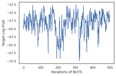
เราตัวอย่างจาก dist การผลิตสถานะเริ่มต้นสำหรับ MCMC จากนั้นเราสามารถกำหนดฟังก์ชันที่ใช้คีย์สุ่มและสถานะเริ่มต้น และสร้างตัวอย่าง 500 รายการจาก No-U-Turn-Sampler (NUTS) โปรดทราบว่าเราสามารถใช้การแปลง JAX เช่น jit รวบรวมตัวอย่างถั่วของเราโดยใช้ XLA
init_key, sample_key = random.split(random.PRNGKey(0))
init_params = tuple(dist.sample(seed=init_key)[:-1])

@jit
def run_chain(key, state):
  kernel = tfp.mcmc.NoUTurnSampler(target_log_prob, 1e-3)
  return tfp.mcmc.sample_chain(500,
      current_state=state,
      kernel=kernel,
      trace_fn=lambda _, results: results.target_log_prob,
      num_burnin_steps=500,
      seed=key)

states, log_probs = run_chain(sample_key, init_params)
plt.figure()
plt.plot(log_probs)
plt.ylabel('Target Log Prob')
plt.xlabel('Iterations of NUTS')
plt.show()
ลองใช้ตัวอย่างของเราในการหาค่าเฉลี่ยแบบจำลองเบย์ (BMA) โดยหาค่าเฉลี่ยความน่าจะเป็นที่คาดการณ์ไว้ของน้ำหนักแต่ละชุด
ขั้นแรก ให้เขียนฟังก์ชันที่สำหรับชุดของพารามิเตอร์ที่กำหนดจะทำให้เกิดความน่าจะเป็นในแต่ละคลาส เราสามารถใช้ dist.sample_distributions ที่จะได้รับการกระจายสุดท้ายในรูปแบบ
def classifier_probs(params):
  dists, _ = dist.sample_distributions(seed=random.PRNGKey(0),
                                       value=params + (None,))
  return dists[-1].distribution.probs_parameter()
เราสามารถ vmap(classifier_probs) มากกว่าชุดของตัวอย่างที่จะได้รับความน่าจะเป็นระดับที่คาดการณ์ไว้สำหรับแต่ละตัวอย่างของเรา จากนั้นเราจะคำนวณความแม่นยำเฉลี่ยในแต่ละตัวอย่าง และความแม่นยำจากค่าเฉลี่ยของแบบจำลองเบย์
all_probs = jit(vmap(classifier_probs))(states)
print('Average accuracy:', jnp.mean(all_probs.argmax(axis=-1) == labels))
print('BMA accuracy:', jnp.mean(all_probs.mean(axis=0).argmax(axis=-1) == labels))
Average accuracy: 0.96952
BMA accuracy: 0.97999996
ดูเหมือนว่า BMA จะลดอัตราความผิดพลาดของเราลงเกือบหนึ่งในสาม!
พื้นฐาน
TFP ใน JAX มี API เหมือนกับ TF ที่แทนการรับวัตถุ TF เช่น tf.Tensor s ยอมรับอนาล็อก JAX ยกตัวอย่างเช่นใดก็ตาม tf.Tensor ถูกนำมาใช้ก่อนหน้านี้เป็น input API ในขณะนี้คาดว่าจะมี JAX DeviceArray แทนที่จะกลับ tf.Tensor วิธี TFP จะกลับ DeviceArray s TFP ใน JAX ยังทำงานร่วมกับโครงสร้างที่ซ้อนกันของวัตถุ JAX เช่นรายการหรือพจนานุกรมของ DeviceArray s
การกระจาย
การแจกแจงของ TFP ส่วนใหญ่ได้รับการสนับสนุนใน JAX โดยมีความหมายที่คล้ายคลึงกันมากกับคู่ของ TF พวกเขายังได้รับการจดทะเบียนเป็น JAX Pytrees เพื่อให้พวกเขาสามารถเป็นปัจจัยการผลิตและผลของฟังก์ชั่น JAX-เปลี่ยน
การแจกแจงพื้นฐาน
log_prob วิธีการสำหรับการกระจายการทำงานเดียวกัน
dist = tfd.Normal(0., 1.)
print(dist.log_prob(0.))
-0.9189385
การสุ่มตัวอย่างจากการกระจายต้องใช้อย่างชัดเจนผ่านใน PRNGKey (หรือรายการของจำนวนเต็ม) ในขณะที่ seed โต้แย้งคำหลัก การไม่ส่งผ่านเมล็ดพันธุ์อย่างชัดเจนจะทำให้เกิดข้อผิดพลาด
tfd.Normal(0., 1.).sample(seed=random.PRNGKey(0))
DeviceArray(-0.20584226, dtype=float32)
ความหมายรูปร่างสำหรับการกระจายยังคงเหมือนเดิมใน JAX ที่กระจายแต่ละคนจะมี event_shape และ batch_shape และการวาดภาพตัวอย่างจำนวนมากจะเพิ่มเพิ่มเติม sample_shape มิติ
ยกตัวอย่างเช่น tfd.MultivariateNormalDiag กับพารามิเตอร์เวกเตอร์จะมีรูปร่างเหตุการณ์เวกเตอร์และรูปทรงชุดที่ว่างเปล่า
dist = tfd.MultivariateNormalDiag(
    loc=jnp.zeros(5),
    scale_diag=jnp.ones(5)
)
print('Event shape:', dist.event_shape)
print('Batch shape:', dist.batch_shape)
Event shape: (5,)
Batch shape: ()
บนมืออื่น ๆ ที่เป็น tfd.Normal แปรกับพาหะจะมีรูปร่างเหตุการณ์สเกลาร์และเวกเตอร์ชุดรูปร่าง
dist = tfd.Normal(
    loc=jnp.ones(5),
    scale=jnp.ones(5),
)
print('Event shape:', dist.event_shape)
print('Batch shape:', dist.batch_shape)
Event shape: ()
Batch shape: (5,)
ความหมายของการ log_prob ตัวอย่างการทำงานเดียวกันใน JAX เกินไป
dist =  tfd.Normal(jnp.zeros(5), jnp.ones(5))
s = dist.sample(sample_shape=(10, 2), seed=random.PRNGKey(0))
print(dist.log_prob(s).shape)

dist =  tfd.Independent(tfd.Normal(jnp.zeros(5), jnp.ones(5)), 1)
s = dist.sample(sample_shape=(10, 2), seed=random.PRNGKey(0))
print(dist.log_prob(s).shape)
(10, 2, 5)
(10, 2)
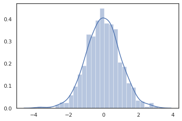
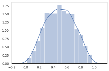
เพราะ JAX DeviceArray s เข้ากันได้กับห้องสมุดเช่น NumPy และ Matplotlib เราสามารถให้อาหารตัวอย่างโดยตรงในฟังก์ชั่นการวางแผน
sns.distplot(tfd.Normal(0., 1.).sample(1000, seed=random.PRNGKey(0)))
plt.show()
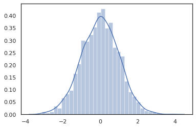
Distribution วิธีการเข้ากันได้กับการเปลี่ยนแปลง JAX
sns.distplot(jit(vmap(lambda key: tfd.Normal(0., 1.).sample(seed=key)))(
    random.split(random.PRNGKey(0), 2000)))
plt.show()
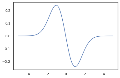
x = jnp.linspace(-5., 5., 100)
plt.plot(x, jit(vmap(grad(tfd.Normal(0., 1.).prob)))(x))
plt.show()
เพราะการกระจาย TFP มีการจดทะเบียนเป็นโหนด pytree JAX เราสามารถเขียนฟังก์ชั่นที่มีการกระจายเป็นปัจจัยการผลิตหรือเอาท์พุทและเปลี่ยนพวกเขาโดยใช้ jit แต่พวกเขายังไม่ได้รับการสนับสนุนเป็นข้อโต้แย้งที่จะ vmap ฟังก์ชั่น -ed
@jit
def random_distribution(key):
  loc_key, scale_key = random.split(key)
  loc, log_scale = random.normal(loc_key), random.normal(scale_key)
  return tfd.Normal(loc, jnp.exp(log_scale))
random_dist = random_distribution(random.PRNGKey(0))
print(random_dist.mean(), random_dist.variance())
0.14389051 0.081832744
การกระจายแบบแปลงร่าง
กระจายเปลี่ยนคือการกระจายตัวอย่างซึ่งจะผ่าน Bijector ยังทำงานออกจากกล่อง (bijectors ทำงานมากเกินไป! ดูด้านล่าง)
dist = tfd.TransformedDistribution(
    tfd.Normal(0., 1.),
    tfb.Sigmoid()
)
sns.distplot(dist.sample(1000, seed=random.PRNGKey(0)))
plt.show()
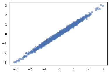
การกระจายร่วม
TFP มี JointDistribution ที่จะช่วยให้การรวมแจกแจงองค์ประกอบเป็นกระจายเดียวมากกว่าหลายตัวแปรสุ่ม ปัจจุบัน TFP ข้อเสนอสามสายพันธุ์หลัก ( JointDistributionSequential , JointDistributionNamed และ JointDistributionCoroutine ) ซึ่งทั้งหมดได้รับการสนับสนุนใน JAX AutoBatched สายพันธุ์นอกจากนี้ยังได้รับการสนับสนุนทั้งหมด
dist = tfd.JointDistributionSequential([
  tfd.Normal(0., 1.),
  lambda x: tfd.Normal(x, 1e-1)
])
plt.scatter(*dist.sample(1000, seed=random.PRNGKey(0)), alpha=0.5)
plt.show()
joint = tfd.JointDistributionNamed(dict(
    e=             tfd.Exponential(rate=1.),
    n=             tfd.Normal(loc=0., scale=2.),
    m=lambda n, e: tfd.Normal(loc=n, scale=e),
    x=lambda    m: tfd.Sample(tfd.Bernoulli(logits=m), 12),
))
joint.sample(seed=random.PRNGKey(0))
{'e': DeviceArray(3.376818, dtype=float32),
 'm': DeviceArray(2.5449684, dtype=float32),
 'n': DeviceArray(-0.6027825, dtype=float32),
 'x': DeviceArray([1, 1, 1, 1, 1, 1, 1, 1, 1, 1, 1, 1], dtype=int32)}
Root = tfd.JointDistributionCoroutine.Root
def model():
  e = yield Root(tfd.Exponential(rate=1.))
  n = yield Root(tfd.Normal(loc=0, scale=2.))
  m = yield tfd.Normal(loc=n, scale=e)
  x = yield tfd.Sample(tfd.Bernoulli(logits=m), 12)

joint = tfd.JointDistributionCoroutine(model)

joint.sample(seed=random.PRNGKey(0))
StructTuple(var0=DeviceArray(0.17315261, dtype=float32), var1=DeviceArray(-3.290489, dtype=float32), var2=DeviceArray(-3.1949058, dtype=float32), var3=DeviceArray([0, 0, 0, 0, 0, 0, 0, 0, 0, 0, 0, 0], dtype=int32))
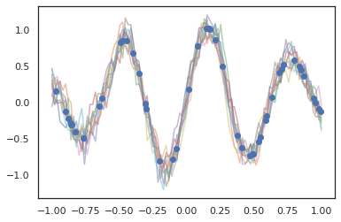
การกระจายอื่น ๆ
กระบวนการเกาส์เซียนยังทำงานในโหมด JAX!
k1, k2, k3 = random.split(random.PRNGKey(0), 3)
observation_noise_variance = 0.01
f = lambda x: jnp.sin(10*x[..., 0]) * jnp.exp(-x[..., 0]**2)
observation_index_points = random.uniform(
    k1, [50], minval=-1.,maxval= 1.)[..., jnp.newaxis]
observations = f(observation_index_points) + tfd.Normal(
    loc=0., scale=jnp.sqrt(observation_noise_variance)).sample(seed=k2)

index_points = jnp.linspace(-1., 1., 100)[..., jnp.newaxis]

kernel = tfpk.ExponentiatedQuadratic(length_scale=0.1)

gprm = tfd.GaussianProcessRegressionModel(
    kernel=kernel,
    index_points=index_points,
    observation_index_points=observation_index_points,
    observations=observations,
    observation_noise_variance=observation_noise_variance)

samples = gprm.sample(10, seed=k3)
for i in range(10):
  plt.plot(index_points, samples[i], alpha=0.5)
plt.plot(observation_index_points, observations, marker='o', linestyle='')
plt.show()
รองรับโมเดล Markov ที่ซ่อนอยู่
initial_distribution = tfd.Categorical(probs=[0.8, 0.2])
transition_distribution = tfd.Categorical(probs=[[0.7, 0.3],
                                                 [0.2, 0.8]])

observation_distribution = tfd.Normal(loc=[0., 15.], scale=[5., 10.])

model = tfd.HiddenMarkovModel(
    initial_distribution=initial_distribution,
    transition_distribution=transition_distribution,
    observation_distribution=observation_distribution,
    num_steps=7)

print(model.mean())
print(model.log_prob(jnp.zeros(7)))
print(model.sample(seed=random.PRNGKey(0)))
[3.       6.       7.5      8.249999 8.625001 8.812501 8.90625 ]
/usr/local/lib/python3.6/dist-packages/tensorflow_probability/substrates/jax/distributions/hidden_markov_model.py:483: UserWarning: HiddenMarkovModel.log_prob in TFP versions < 0.12.0 had a bug in which the transition model was applied prior to the initial step. This bug has been fixed. You may observe a slight change in behavior.
  'HiddenMarkovModel.log_prob in TFP versions < 0.12.0 had a bug '
-19.855635
[ 1.3641367  0.505798   1.3626463  3.6541772  2.272286  15.10309
 22.794212 ]
กระจายน้อยเช่น PixelCNN ยังไม่สนับสนุนเนื่องจากการอ้างอิงที่เข้มงวดเกี่ยวกับ TensorFlow หรือ XLA กันไม่ได้
Bijectors
bijectors ของ TFP ส่วนใหญ่รองรับ JAX แล้ววันนี้!
tfb.Exp().inverse(1.)
DeviceArray(0., dtype=float32)
bij = tfb.Shift(1.)(tfb.Scale(3.))
print(bij.forward(jnp.ones(5)))
print(bij.inverse(jnp.ones(5)))
[4. 4. 4. 4. 4.]
[0. 0. 0. 0. 0.]
b = tfb.FillScaleTriL(diag_bijector=tfb.Exp(), diag_shift=None)
print(b.forward(x=[0., 0., 0.]))
print(b.inverse(y=[[1., 0], [.5, 2]]))
[[1. 0.]
 [0. 1.]]
[0.6931472 0.5       0.       ]
b = tfb.Chain([tfb.Exp(), tfb.Softplus()])
# or:
# b = tfb.Exp()(tfb.Softplus())
print(b.forward(-jnp.ones(5)))
[1.3678794 1.3678794 1.3678794 1.3678794 1.3678794]
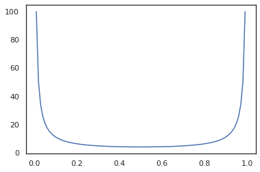
Bijectors เข้ากันได้กับการเปลี่ยนแปลง JAX เช่น jit , grad และ vmap
jit(vmap(tfb.Exp().inverse))(jnp.arange(4.))
DeviceArray([ -inf, 0. , 0.6931472, 1.0986123], dtype=float32)
x = jnp.linspace(0., 1., 100)
plt.plot(x, jit(grad(lambda x: vmap(tfb.Sigmoid().inverse)(x).sum()))(x))
plt.show()
bijectors บางอย่างเช่น RealNVP และ FFJORD ยังไม่สนับสนุน
MCMC
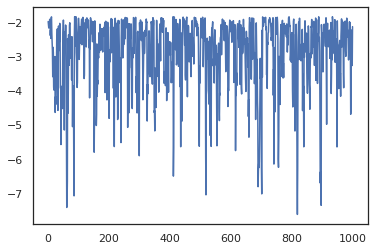
เราได้รังเพลิง tfp.mcmc เพื่อ JAX เป็นอย่างดีเพื่อให้เราสามารถเรียกใช้ขั้นตอนวิธีการเช่นมิล Monte Carlo (HMC) และ No-U-Turn-Sampler (ถั่ว) ใน JAX
target_log_prob = tfd.MultivariateNormalDiag(jnp.zeros(2), jnp.ones(2)).log_prob
ซึ่งแตกต่างจาก TFP ใน TF เราจะต้องผ่านการ PRNGKey เข้า sample_chain ใช้ seed โต้แย้งคำหลัก
def run_chain(key, state):
  kernel = tfp.mcmc.NoUTurnSampler(target_log_prob, 1e-1)
  return tfp.mcmc.sample_chain(1000,
      current_state=state,
      kernel=kernel,
      trace_fn=lambda _, results: results.target_log_prob,
      seed=key)
states, log_probs = jit(run_chain)(random.PRNGKey(0), jnp.zeros(2))
plt.figure()
plt.scatter(*states.T, alpha=0.5)
plt.figure()
plt.plot(log_probs)
plt.show()
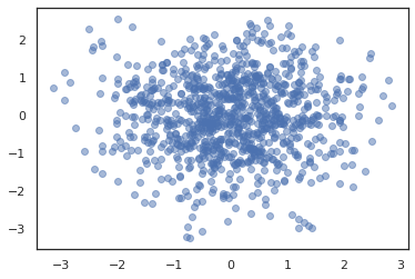
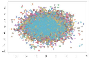
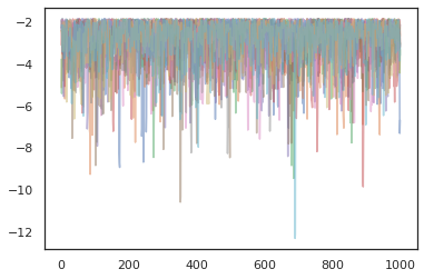
เมื่อต้องการเรียกใช้โซ่หลายรายการเราทั้งสามารถส่งผ่านชุดของรัฐเข้าไป sample_chain หรือการใช้ vmap (แม้ว่าเรายังไม่ได้สำรวจความแตกต่างของผลการดำเนินงานระหว่างทั้งสองวิธี)
states, log_probs = jit(run_chain)(random.PRNGKey(0), jnp.zeros([10, 2]))
plt.figure()
for i in range(10):
  plt.scatter(*states[:, i].T, alpha=0.5)
plt.figure()
for i in range(10):
  plt.plot(log_probs[:, i], alpha=0.5)
plt.show()
เครื่องมือเพิ่มประสิทธิภาพ
TFP บน JAX รองรับเครื่องมือเพิ่มประสิทธิภาพที่สำคัญบางตัว เช่น BFGS และ L-BFGS มาตั้งค่าฟังก์ชันการสูญเสียกำลังสองที่ปรับขนาดอย่างง่ายกัน
minimum = jnp.array([1.0, 1.0])  # The center of the quadratic bowl.
scales = jnp.array([2.0, 3.0])  # The scales along the two axes.

# The objective function and the gradient.
def quadratic_loss(x):
  return jnp.sum(scales * jnp.square(x - minimum))

start = jnp.array([0.6, 0.8])  # Starting point for the search.
BFGS สามารถค้นหาความสูญเสียขั้นต่ำนี้ได้
optim_results = tfp.optimizer.bfgs_minimize(
    value_and_grad(quadratic_loss), initial_position=start, tolerance=1e-8)

# Check that the search converged
assert(optim_results.converged)
# Check that the argmin is close to the actual value.
np.testing.assert_allclose(optim_results.position, minimum)
# Print out the total number of function evaluations it took. Should be 5.
print("Function evaluations: %d" % optim_results.num_objective_evaluations)
Function evaluations: 5
L-BFGS ก็ทำได้เช่นกัน
optim_results = tfp.optimizer.lbfgs_minimize(
    value_and_grad(quadratic_loss), initial_position=start, tolerance=1e-8)

# Check that the search converged
assert(optim_results.converged)
# Check that the argmin is close to the actual value.
np.testing.assert_allclose(optim_results.position, minimum)
# Print out the total number of function evaluations it took. Should be 5.
print("Function evaluations: %d" % optim_results.num_objective_evaluations)
Function evaluations: 5
เพื่อ vmap L-BFGS ให้ชุดของฟังก์ชั่นที่เพิ่มประสิทธิภาพการขาดทุนสำหรับจุดเริ่มต้นเดียว
def optimize_single(start):
  return tfp.optimizer.lbfgs_minimize(
      value_and_grad(quadratic_loss), initial_position=start, tolerance=1e-8)

all_results = jit(vmap(optimize_single))(
    random.normal(random.PRNGKey(0), (10, 2)))
assert all(all_results.converged)
for i in range(10):
  np.testing.assert_allclose(optim_results.position[i], minimum)
print("Function evaluations: %s" % all_results.num_objective_evaluations)
Function evaluations: [6 6 9 6 6 8 6 8 5 9]
คำเตือน
มีความแตกต่างพื้นฐานบางอย่างระหว่าง TF และ JAX ลักษณะการทำงานของ TFP บางอย่างจะแตกต่างกันระหว่างพื้นผิวทั้งสอง และไม่รองรับฟังก์ชันการทำงานทั้งหมด ตัวอย่างเช่น,
- TFP ใน JAX ไม่สนับสนุนอะไรเช่น
tf.Variableตั้งแต่ไม่มีอะไรเหมือนมันมีอยู่ใน JAX นอกจากนี้ยังหมายความสาธารณูปโภคเช่นtfp.util.TransformedVariableยังไม่ได้รับการสนับสนุนอย่างใดอย่างหนึ่ง -
tfp.layersไม่ได้รับการสนับสนุนในส่วนหลัง ๆ เนื่องจากการพึ่งพา Keras และtf.Variables -
tfp.math.minimizeไม่ทำงานใน TFP ใน JAX เพราะการพึ่งพาtf.Variable - ด้วย TFP บน JAX รูปร่างเทนเซอร์จะเป็นค่าจำนวนเต็มที่เป็นรูปธรรมเสมอ และจะไม่เป็นที่รู้จัก/เป็นไดนามิกเหมือนใน TFP บน TF
- การสุ่มหลอกได้รับการจัดการแตกต่างกันใน TF และ JAX (ดูภาคผนวก)
- ห้องสมุดใน
tfp.experimentalจะไม่รับประกันว่าจะมีอยู่ในสารตั้งต้น JAX - กฎการเลื่อนระดับ Dtype นั้นแตกต่างกันระหว่าง TF และ JAX TFP บน JAX พยายามเคารพความหมาย dtype ของ TF ภายในเพื่อความสอดคล้อง
- Bijectors ยังไม่ได้ลงทะเบียนเป็น JAX pytrees
หากต้องการดูรายการที่สมบูรณ์ของสิ่งที่ได้รับการสนับสนุนใน TFP ใน JAX, โปรดดูที่ เอกสาร API
บทสรุป
เราได้ย้ายคุณสมบัติมากมายของ TFP ไปยัง JAX และรู้สึกตื่นเต้นที่จะได้เห็นสิ่งที่ทุกคนจะสร้าง ฟังก์ชันบางอย่างยังไม่ได้รับการสนับสนุน ถ้าเราได้พลาดสิ่งที่สำคัญกับคุณ (หรือถ้าคุณพบข้อผิดพลาด!) โปรดติดต่อเรา - คุณสามารถส่งอีเมล tfprobability@tensorflow.org หรือไฟล์ปัญหาใน repo Github ของเรา
ภาคผนวก: การสุ่มเทียมใน JAX
JAX หมายเลข pseudorandom รุ่น (PRNG) รุ่นไร้สัญชาติ ต่างจากโมเดล stateful ไม่มีสถานะโกลบอลที่ไม่แน่นอนที่วิวัฒนาการหลังจากการสุ่มแต่ละครั้ง ในรูปแบบ JAX ของเราเริ่มต้นด้วยคีย์ PRNG ซึ่งทำหน้าที่เหมือนคู่ของจำนวนเต็ม 32 บิต เราสามารถสร้างปุ่มเหล่านี้โดยใช้ jax.random.PRNGKey
key = random.PRNGKey(0)  # Creates a key with value [0, 0]
print(key)
[0 0]
ฟังก์ชั่นสุ่มใน JAX ใช้กุญแจสำคัญในการผลิต deterministically ตัวแปรสุ่มหมายถึงพวกเขาไม่ควรนำมาใช้อีกครั้ง ตัวอย่างเช่นเราสามารถใช้ key ที่จะลิ้มลองค่าการกระจายตามปกติ แต่เราไม่ควรใช้ key อีกครั้งอื่น ๆ นอกจากนี้การส่งผ่านค่าเดียวกันใน random.normal จะผลิตค่าเดียวกัน
print(random.normal(key))
-0.20584226
แล้วเราจะวาดตัวอย่างหลายตัวอย่างจากคีย์เดียวได้อย่างไร คำตอบคือแยกที่สำคัญ ความคิดพื้นฐานคือการที่เราสามารถแยก PRNGKey ออกเป็นหลาย ๆ และแต่ละคีย์ใหม่สามารถรักษาได้เป็นแหล่งที่เป็นอิสระจากการสุ่ม
key1, key2 = random.split(key, num=2)
print(key1, key2)
[4146024105 967050713] [2718843009 1272950319]
การแยกคีย์เป็นสิ่งที่กำหนดได้ แต่มีความโกลาหล ดังนั้นตอนนี้แต่ละคีย์ใหม่สามารถใช้เพื่อสุ่มตัวอย่างที่แตกต่างกันได้
print(random.normal(key1), random.normal(key2))
0.14389051 -1.2515389
สำหรับรายละเอียดเพิ่มเติมเกี่ยวกับรูปแบบที่สำคัญแยก JAX ของกำหนดดู คำแนะนำนี้