| | |  ดูแหล่งที่มาบน GitHub ดูแหล่งที่มาบน GitHub | |
นี่คือพอร์ตความน่าจะเป็นของ TensorFlow ของเอกสารฉบับวันที่ 16 มีนาคม 2020 โดย Li et al เราทำซ้ำวิธีการและผลลัพธ์ของผู้เขียนดั้งเดิมอย่างซื่อสัตย์บนแพลตฟอร์ม TensorFlow Probability โดยแสดงความสามารถบางอย่างของ TFP ในการสร้างแบบจำลองทางระบาดวิทยาสมัยใหม่ การย้ายไปยัง TensorFlow ทำให้เรามีความเร็วเพิ่มขึ้นประมาณ 10 เท่าเมื่อเทียบกับรหัส Matlab ดั้งเดิม และเนื่องจากความน่าจะเป็นของ TensorFlow รองรับการคำนวณแบบแบทช์แบบเวคเตอร์อย่างแพร่หลาย จึงปรับขนาดเป็นการจำลองแบบอิสระหลายร้อยรายการในเกณฑ์ดี
กระดาษต้นฉบับ
Ruiyun Li, Sen Pei, Bin Chen, Yimeng Song, Tao Zhang, Wan Yang และ Jeffrey Shaman การติดเชื้อที่ไม่มีเอกสารสำคัญช่วยให้การแพร่กระจายของ coronavirus ใหม่ (SARS-CoV2) เป็นไปอย่างรวดเร็ว (2020), ดอย: https://doi.org/10.1126/science.abb3221
บทคัดย่อ:. "การประเมินความชุกและ contagiousness ของนวนิยาย coronavirus (โรคซาร์ส CoV2) การติดเชื้อที่ไม่มีเอกสารเป็นสิ่งสำคัญสำหรับการทำความเข้าใจความชุกและมีศักยภาพในการแพร่ระบาดของโรคนี้ที่นี่เราใช้การสังเกตของการติดเชื้อรายงานภายในประเทศจีนร่วมกับข้อมูลการเคลื่อนไหวเป็น โมเดล metapopulation แบบไดนามิกของเครือข่ายและการอนุมานแบบเบย์เพื่อสรุปลักษณะทางระบาดวิทยาที่สำคัญที่เกี่ยวข้องกับ SARS-CoV2 รวมถึงส่วนของการติดเชื้อที่ไม่มีเอกสารและการติดต่อ เราประมาณว่า 86% ของการติดเชื้อทั้งหมดไม่มีเอกสาร (95% CI: [82%–90%] ) ก่อนวันที่ 23 มกราคม 2020 ข้อจำกัดการเดินทาง ต่อคน อัตราการแพร่กระจายของการติดเชื้อที่ไม่มีเอกสารเป็น 55% ของการติดเชื้อในเอกสาร ([46%–62 เปอร์เซ็นต์]) แต่เนื่องจากจำนวนที่มากขึ้น การติดเชื้อที่ไม่มีเอกสารจึงเป็นแหล่งที่มาของการติดเชื้อ 79 % ของกรณีที่มีเอกสาร ผลการวิจัยเหล่านี้อธิบายการแพร่กระจายอย่างรวดเร็วของ SARS-CoV2 ทางภูมิศาสตร์และบ่งชี้ว่าการกักกันไวรัสนี้จะเป็นสิ่งที่ท้าทายอย่างยิ่ง"
การเชื่อมโยง Github รหัสและข้อมูลที่
ภาพรวม
รูปแบบคือ รูปแบบการเกิดโรค compartmental มีช่องสำหรับ "อ่อนแอ", "สัมผัส" (ติดเชื้อ แต่ยังไม่ได้ติดเชื้อ), "ไม่เคยมีเอกสารติดเชื้อ" และ "ในที่สุดเอกสารการติดเชื้อ" มีลักษณะเด่นสองประการ: ช่องแบ่งสำหรับเมืองจีน 375 เมืองแต่ละแห่ง โดยมีการสันนิษฐานว่าผู้คนเดินทางจากเมืองหนึ่งไปยังอีกเมืองหนึ่งอย่างไร และความล่าช้าในการรายงานการติดเชื้อเพื่อให้กลายเป็นกรณีที่ว่า "ในที่สุดเอกสารการติดเชื้อ" ในวันที่ \(t\) ไม่ปรากฏขึ้นในกรณีที่นับสังเกตจนกระทั่งวันต่อมาสุ่ม
แบบจำลองนี้อนุมานว่าคดีที่ไม่ได้รับการจัดทำเป็นเอกสารจะสิ้นสุดลงโดยไม่มีเอกสารประกอบโดยอาการรุนแรงขึ้น และทำให้ผู้อื่นติดเชื้อในอัตราที่ต่ำกว่า พารามิเตอร์หลักที่น่าสนใจในเอกสารต้นฉบับคือสัดส่วนของกรณีที่ยังไม่มีเอกสาร เพื่อประเมินทั้งขอบเขตของการติดเชื้อที่มีอยู่ และผลกระทบของการแพร่ระบาดที่ไม่มีเอกสารเกี่ยวกับการแพร่กระจายของโรค
colab นี้มีโครงสร้างเป็นคำแนะนำแบบโค้ดในรูปแบบจากล่างขึ้นบน เพื่อที่เราจะ
- กลืนกินและตรวจสอบข้อมูลโดยสังเขป
- กำหนดพื้นที่สถานะและไดนามิกของโมเดล
- สร้างชุดฟังก์ชันสำหรับการอนุมานในแบบจำลองตาม Li et al และ
- เรียกพวกเขาและตรวจสอบผลลัพธ์ สปอยเลอร์: พวกเขาออกมาเหมือนกับกระดาษ
การติดตั้งและการนำเข้า Python
pip3 install -q tf-nightly tfp-nightly
import collections
import io
import requests
import time
import zipfile

import matplotlib.pyplot as plt
import numpy as np
import pandas as pd

import tensorflow.compat.v2 as tf
import tensorflow_probability as tfp
from tensorflow_probability.python.internal import samplers

tfd = tfp.distributions
tfes = tfp.experimental.sequential
นำเข้าข้อมูล
มานำเข้าข้อมูลจาก github และตรวจสอบข้อมูลบางส่วนกัน
r = requests.get('https://raw.githubusercontent.com/SenPei-CU/COVID-19/master/Data.zip')
z = zipfile.ZipFile(io.BytesIO(r.content))
z.extractall('/tmp/')
raw_incidence = pd.read_csv('/tmp/data/Incidence.csv')
raw_mobility = pd.read_csv('/tmp/data/Mobility.csv')
raw_population = pd.read_csv('/tmp/data/pop.csv')
ด้านล่างเราจะดูจำนวนอุบัติการณ์ดิบต่อวัน เราสนใจมากที่สุดในช่วง 14 วันแรก (10 มกราคม ถึง 23 มกราคม) เนื่องจากมีการจำกัดการเดินทางในวันที่ 23 บทความนี้กล่าวถึงเรื่องนี้โดยการสร้างแบบจำลองระหว่างวันที่ 10-23 ม.ค. และ 23 ม.ค. แยกกัน โดยมีพารามิเตอร์ต่างกัน เราจะจำกัดการสืบพันธุ์ของเราให้อยู่ในช่วงเวลาก่อนหน้าเท่านั้น
raw_incidence.drop('Date', axis=1)  # The 'Date' column is all 1/18/21
# Luckily the days are in order, starting on January 10th, 2020.
มาตรวจสุขภาพกัน-ตรวจนับอุบัติการณ์เมืองอู่ฮั่นกันเถอะ
plt.plot(raw_incidence.Wuhan, '.-')
plt.title('Wuhan incidence counts over 1/10/20 - 02/08/20')
plt.show()
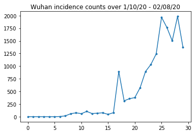
จนถึงตอนนี้ดีมาก ตอนนี้นับจำนวนประชากรเริ่มต้น
raw_population
ตรวจสอบและบันทึกว่ารายการใดคือหวู่ฮั่น
raw_population['City'][169]
'Wuhan'
WUHAN_IDX = 169
และที่นี่เราเห็นเมทริกซ์ความคล่องตัวระหว่างเมืองต่างๆ นี่คือตัวแทนจำนวนคนที่ย้ายไปมาระหว่างเมืองต่างๆ ใน 14 วันแรก มาจากบันทึก GPS ของ Tencent สำหรับเทศกาลตรุษจีนปี 2018 Li et al, รูปแบบการเคลื่อนไหวในช่วงฤดูกาล 2020 เป็นที่รู้จักบางคน (อาจมีการอนุมาน) ปัจจัยคง \(\theta\) ครั้งนี้
raw_mobility
สุดท้ายนี้ มาประมวลผลล่วงหน้าทั้งหมดนี้เป็นอาร์เรย์จำนวนมากที่เราสามารถใช้ได้
# The given populations are only "initial" because of intercity mobility during
# the holiday season.
initial_population = raw_population['Population'].to_numpy().astype(np.float32)
แปลงข้อมูลการเคลื่อนที่เป็นเมตริกซ์รูป [L, L, T] โดยที่ L คือจำนวนตำแหน่ง และ T คือจำนวนขั้นของเวลา
daily_mobility_matrices = []
for i in range(1, 15):
  day_mobility = raw_mobility[raw_mobility['Day'] == i]

  # Make a matrix of daily mobilities.
  z = pd.crosstab(
      day_mobility.Origin,
      day_mobility.Destination,
      values=day_mobility['Mobility Index'], aggfunc='sum', dropna=False)

  # Include every city, even if there are no rows for some in the raw data on
  # some day.  This uses the sort order of `raw_population`.
  z = z.reindex(index=raw_population['City'], columns=raw_population['City'],
                fill_value=0)
  # Finally, fill any missing entries with 0. This means no mobility.
  z = z.fillna(0)
  daily_mobility_matrices.append(z.to_numpy())

mobility_matrix_over_time = np.stack(daily_mobility_matrices, axis=-1).astype(
    np.float32)
ขั้นสุดท้ายนำการติดเชื้อที่สังเกตได้และสร้างตาราง [L, T]
# Remove the date parameter and take the first 14 days.
observed_daily_infectious_count = raw_incidence.to_numpy()[:14, 1:]
observed_daily_infectious_count = np.transpose(
    observed_daily_infectious_count).astype(np.float32)
และตรวจสอบอีกครั้งว่าเราได้รูปทรงตามที่เราต้องการแล้ว เรากำลังดำเนินการกับ 375 เมือง 14 วัน
print('Mobility Matrix over time should have shape (375, 375, 14): {}'.format(
    mobility_matrix_over_time.shape))
print('Observed Infectious should have shape (375, 14): {}'.format(
    observed_daily_infectious_count.shape))
print('Initial population should have shape (375): {}'.format(
    initial_population.shape))
Mobility Matrix over time should have shape (375, 375, 14): (375, 375, 14)
Observed Infectious should have shape (375, 14): (375, 14)
Initial population should have shape (375): (375,)
การกำหนดสถานะและพารามิเตอร์
มาเริ่มกำหนดแบบจำลองของเรากัน รูปแบบที่เรากำลังทำซ้ำเป็นตัวแปรของ รุ่น SEIR ในกรณีนี้ เรามีสถานะที่แปรผันตามเวลาดังต่อไปนี้:
- \(S\): จำนวนคนที่ไวต่อการเกิดโรคในแต่ละเมือง
- \(E\): จำนวนของผู้คนในแต่ละเมืองสัมผัสกับโรคติดเชื้อ แต่ไม่เลย ในทางชีววิทยา สิ่งนี้สอดคล้องกับการติดโรค โดยที่คนที่สัมผัสทั้งหมดจะกลายเป็นคนติดเชื้อในที่สุด
- \(I^u\): จำนวนของผู้คนในแต่ละเมืองที่มีการติดเชื้อ แต่ไม่มีเอกสาร ในแบบจำลองนี้ แท้จริงแล้วหมายความว่า "จะไม่มีการจัดทำเป็นเอกสาร"
- \(I^r\): จำนวนของผู้คนในแต่ละเมืองที่มีการติดเชื้อและจัดทำเอกสารดังกล่าว Li et al, รายงานความล่าช้ารูปแบบเพื่อให้ \(I^r\) จริงสอดคล้องกับสิ่งที่ชอบ "กรณีเป็นพออย่างรุนแรงต่อการได้รับการบันทึกที่จุดในอนาคตบาง"
ดังที่เราเห็นด้านล่าง เราจะอนุมานสถานะเหล่านี้โดยเรียกใช้ Kalman Filter ที่ปรับ Ensemble (EAKF) ไปข้างหน้าทันเวลา เวกเตอร์สถานะของ EAKF เป็นเวกเตอร์ที่จัดทำดัชนีเมืองหนึ่งรายการสำหรับแต่ละปริมาณเหล่านี้
โมเดลมีพารามิเตอร์ที่ไม่เปลี่ยนแปลงตามเวลาสากลที่อนุมานได้ดังต่อไปนี้:
- \(\beta\): อัตราการส่งผ่านเนื่องจากบุคคลที่ติดเชื้อเอกสาร
- \(\mu\): อัตราการส่งญาติเนื่องจากบุคคลที่ไม่มีเอกสารติดเชื้อ นี้จะทำหน้าที่ผ่านผลิตภัณฑ์ \(\mu \beta\)
- \(\theta\): ปัจจัยระหว่างการเคลื่อนย้าย นี่เป็นปัจจัยที่มากกว่า 1 ในการแก้ไขสำหรับการรายงานข้อมูลการเคลื่อนย้ายที่ต่ำกว่าความเป็นจริง (และสำหรับการเติบโตของประชากรตั้งแต่ปี 2018 ถึง 2020)
- \(Z\): ระยะฟักตัวเฉลี่ย (เช่นเวลาในการ "สัมผัส" รัฐ)
- \(\alpha\): นี่คือส่วนของการติดเชื้อรุนแรงพอที่จะเป็น (ในที่สุด) เอกสาร
- \(D\): ระยะเวลาเฉลี่ยของการติดเชื้อ (เช่นเวลาทั้งในรัฐ "ติดเชื้อ")
เราจะอนุมานค่าประมาณจุดสำหรับพารามิเตอร์เหล่านี้ด้วยการวนซ้ำการกรองซ้ำรอบ EAKF สำหรับสถานะต่างๆ
โมเดลยังขึ้นอยู่กับค่าคงที่ที่ไม่ได้อนุมานด้วย:
- \(M\): ในระหว่างการเคลื่อนไหวเมทริกซ์ นี่เป็นเวลาที่แตกต่างกันและถือว่าได้รับ จำได้ว่ามันปรับขนาดโดยสรุปพารามิเตอร์ \(\theta\) เพื่อให้การเคลื่อนไหวของประชากรที่เกิดขึ้นจริงระหว่างเมือง
- \(N\): จำนวนของผู้คนในแต่ละเมือง ประชากรเริ่มต้นถูกนำมาเป็นรับและเวลาการเปลี่ยนแปลงของประชากรคำนวณจากตัวเลขการเคลื่อนไหว \(\theta M\)
ขั้นแรก เราให้โครงสร้างข้อมูลบางอย่างแก่ตัวเองสำหรับเก็บสถานะและพารามิเตอร์ของเรา
SEIRComponents = collections.namedtuple(
  typename='SEIRComponents',
  field_names=[
    'susceptible',              # S
    'exposed',                  # E
    'documented_infectious',    # I^r
    'undocumented_infectious',  # I^u
    # This is the count of new cases in the "documented infectious" compartment.
    # We need this because we will introduce a reporting delay, between a person
    # entering I^r and showing up in the observable case count data.
    # This can't be computed from the cumulative `documented_infectious` count,
    # because some portion of that population will move to the 'recovered'
    # state, which we aren't tracking explicitly.
    'daily_new_documented_infectious'])

ModelParams = collections.namedtuple(
    typename='ModelParams',
    field_names=[
      'documented_infectious_tx_rate',             # Beta
      'undocumented_infectious_tx_relative_rate',  # Mu
      'intercity_underreporting_factor',           # Theta
      'average_latency_period',                    # Z
      'fraction_of_documented_infections',         # Alpha
      'average_infection_duration'                 # D
    ]
)
นอกจากนี้เรายังกำหนดขอบเขตของ Li et al สำหรับค่าของพารามิเตอร์
PARAMETER_LOWER_BOUNDS = ModelParams(
    documented_infectious_tx_rate=0.8,
    undocumented_infectious_tx_relative_rate=0.2,
    intercity_underreporting_factor=1.,
    average_latency_period=2.,
    fraction_of_documented_infections=0.02,
    average_infection_duration=2.
)

PARAMETER_UPPER_BOUNDS = ModelParams(
    documented_infectious_tx_rate=1.5,
    undocumented_infectious_tx_relative_rate=1.,
    intercity_underreporting_factor=1.75,
    average_latency_period=5.,
    fraction_of_documented_infections=1.,
    average_infection_duration=5.
)
SEIR Dynamics
ที่นี่เรากำหนดความสัมพันธ์ระหว่างพารามิเตอร์และสถานะ
สมการไดนามิกของเวลาจาก Li et al (วัสดุเสริม eqns 1-5) มีดังนี้:
\(\frac{dS_i}{dt} = -\beta \frac{S_i I_i^r}{N_i} - \mu \beta \frac{S_i I_i^u}{N_i} + \theta \sum_k \frac{M_{ij} S_j}{N_j - I_j^r} - + \theta \sum_k \frac{M_{ji} S_j}{N_i - I_i^r}\)
\(\frac{dE_i}{dt} = \beta \frac{S_i I_i^r}{N_i} + \mu \beta \frac{S_i I_i^u}{N_i} -\frac{E_i}{Z} + \theta \sum_k \frac{M_{ij} E_j}{N_j - I_j^r} - + \theta \sum_k \frac{M_{ji} E_j}{N_i - I_i^r}\)
\(\frac{dI^r_i}{dt} = \alpha \frac{E_i}{Z} - \frac{I_i^r}{D}\)
\(\frac{dI^u_i}{dt} = (1 - \alpha) \frac{E_i}{Z} - \frac{I_i^u}{D} + \theta \sum_k \frac{M_{ij} I_j^u}{N_j - I_j^r} - + \theta \sum_k \frac{M_{ji} I^u_j}{N_i - I_i^r}\)
\(N_i = N_i + \theta \sum_j M_{ij} - \theta \sum_j M_{ji}\)
เป็นคำเตือนที่ \(i\) และ \(j\) เมืองดัชนีห้อย สมการเหล่านี้จำลองวิวัฒนาการเวลาของโรคผ่าน
- ติดต่อกับบุคคลที่ติดเชื้อที่นำไปสู่การติดเชื้อมากขึ้น
- การลุกลามของโรคจาก "สัมผัส" ไปสู่สถานะ "ติดเชื้อ" อย่างใดอย่างหนึ่ง
- การลุกลามของโรคจากสถานะ "ติดเชื้อ" ไปสู่การฟื้นตัว ซึ่งเราจำลองโดยการกำจัดออกจากประชากรที่เป็นแบบจำลอง
- การเคลื่อนย้ายระหว่างเมือง รวมทั้งบุคคลที่สัมผัสหรือไม่ได้รับเอกสาร และ
- การเปลี่ยนแปลงเวลาของประชากรในเมืองในแต่ละวันผ่านการเคลื่อนย้ายระหว่างเมือง
ตาม Li et al เราคิดว่าคนที่มีอาการรุนแรงมากพอที่จะรายงานได้ในที่สุดจะไม่เดินทางระหว่างเมือง
นอกจากนี้ ตาม Li et al เราถือว่าพลวัตเหล่านี้อยู่ภายใต้เสียงปัวซองที่ชาญฉลาด กล่าวคือ แต่ละเทอมเป็นอัตราของปัวซอง ซึ่งเป็นตัวอย่างที่ทำให้เกิดการเปลี่ยนแปลงที่แท้จริง สัญญาณรบกวนของปัวซองนั้นฉลาดตามคำศัพท์เพราะการลบตัวอย่างปัวซอง (ตรงข้ามกับการบวก) ไม่ได้ให้ผลลัพธ์แบบกระจายปัวซอง
เราจะพัฒนาไดนามิกเหล่านี้ไปข้างหน้าอย่างทันท่วงทีด้วยผู้รวบรวม Runge-Kutta ลำดับที่สี่สุดคลาสสิก แต่ก่อนอื่น เรามากำหนดฟังก์ชันที่คำนวณกันก่อน (รวมถึงการสุ่มตัวอย่างสัญญาณรบกวนปัวซอง)
def sample_state_deltas(
    state, population, mobility_matrix, params, seed, is_deterministic=False):
  """Computes one-step change in state, including Poisson sampling.

  Note that this is coded to support vectorized evaluation on arbitrary-shape
  batches of states.  This is useful, for example, for running multiple
  independent replicas of this model to compute credible intervals for the
  parameters.  We refer to the arbitrary batch shape with the conventional
  `B` in the parameter documentation below.  This function also, of course,
  supports broadcasting over the batch shape.

  Args:
    state: A `SEIRComponents` tuple with fields Tensors of shape
      B + [num_locations] giving the current disease state.
    population: A Tensor of shape B + [num_locations] giving the current city
      populations.
    mobility_matrix: A Tensor of shape B + [num_locations, num_locations] giving
      the current baseline inter-city mobility.
    params: A `ModelParams` tuple with fields Tensors of shape B giving the
      global parameters for the current EAKF run.
    seed: Initial entropy for pseudo-random number generation.  The Poisson
      sampling is repeatable by supplying the same seed.
    is_deterministic: A `bool` flag to turn off Poisson sampling if desired.

  Returns:
    delta: A `SEIRComponents` tuple with fields Tensors of shape
      B + [num_locations] giving the one-day changes in the state, according
      to equations 1-4 above (including Poisson noise per Li et al).
  """
  undocumented_infectious_fraction = state.undocumented_infectious / population
  documented_infectious_fraction = state.documented_infectious / population

  # Anyone not documented as infectious is considered mobile
  mobile_population = (population - state.documented_infectious)
  def compute_outflow(compartment_population):
    raw_mobility = tf.linalg.matvec(
        mobility_matrix, compartment_population / mobile_population)
    return params.intercity_underreporting_factor * raw_mobility
  def compute_inflow(compartment_population):
    raw_mobility = tf.linalg.matmul(
        mobility_matrix,
        (compartment_population / mobile_population)[..., tf.newaxis],
        transpose_a=True)
    return params.intercity_underreporting_factor * tf.squeeze(
        raw_mobility, axis=-1)

  # Helper for sampling the Poisson-variate terms.
  seeds = samplers.split_seed(seed, n=11)
  if is_deterministic:
    def sample_poisson(rate):
      return rate
  else:
    def sample_poisson(rate):
      return tfd.Poisson(rate=rate).sample(seed=seeds.pop())

  # Below are the various terms called U1-U12 in the paper. We combined the
  # first two, which should be fine; both are poisson so their sum is too, and
  # there's no risk (as there could be in other terms) of going negative.
  susceptible_becoming_exposed = sample_poisson(
      state.susceptible *
      (params.documented_infectious_tx_rate *
       documented_infectious_fraction +
       (params.undocumented_infectious_tx_relative_rate *
        params.documented_infectious_tx_rate) *
       undocumented_infectious_fraction))  # U1 + U2

  susceptible_population_inflow = sample_poisson(
      compute_inflow(state.susceptible))  # U3
  susceptible_population_outflow = sample_poisson(
      compute_outflow(state.susceptible))  # U4

  exposed_becoming_documented_infectious = sample_poisson(
      params.fraction_of_documented_infections *
      state.exposed / params.average_latency_period)  # U5
  exposed_becoming_undocumented_infectious = sample_poisson(
      (1 - params.fraction_of_documented_infections) *
      state.exposed / params.average_latency_period)  # U6

  exposed_population_inflow = sample_poisson(
      compute_inflow(state.exposed))  # U7
  exposed_population_outflow = sample_poisson(
      compute_outflow(state.exposed))  # U8

  documented_infectious_becoming_recovered = sample_poisson(
      state.documented_infectious /
      params.average_infection_duration)  # U9
  undocumented_infectious_becoming_recovered = sample_poisson(
      state.undocumented_infectious /
      params.average_infection_duration)  # U10

  undocumented_infectious_population_inflow = sample_poisson(
      compute_inflow(state.undocumented_infectious))  # U11
  undocumented_infectious_population_outflow = sample_poisson(
      compute_outflow(state.undocumented_infectious))  # U12

  # The final state_deltas
  return SEIRComponents(
      # Equation [1]
      susceptible=(-susceptible_becoming_exposed +
                   susceptible_population_inflow +
                   -susceptible_population_outflow),
      # Equation [2]
      exposed=(susceptible_becoming_exposed +
               -exposed_becoming_documented_infectious +
               -exposed_becoming_undocumented_infectious +
               exposed_population_inflow +
               -exposed_population_outflow),
      # Equation [3]
      documented_infectious=(
          exposed_becoming_documented_infectious +
          -documented_infectious_becoming_recovered),
      # Equation [4]
      undocumented_infectious=(
          exposed_becoming_undocumented_infectious +
          -undocumented_infectious_becoming_recovered +
          undocumented_infectious_population_inflow +
          -undocumented_infectious_population_outflow),
      # New to-be-documented infectious cases, subject to the delayed
      # observation model.
      daily_new_documented_infectious=exposed_becoming_documented_infectious)
นี่คือผู้รวบรวม นี่คือมาตรฐานสมบูรณ์ยกเว้นสำหรับการส่งผ่านเมล็ด PRNG ผ่านไป sample_state_deltas ทำงานที่จะได้รับอิสระ Poisson เสียงในแต่ละขั้นตอนบางส่วนว่าวิธีการ Runge-Kutta เรียกร้องให้
@tf.function(autograph=False)
def rk4_one_step(state, population, mobility_matrix, params, seed):
  """Implement one step of RK4, wrapped around a call to sample_state_deltas."""
  # One seed for each RK sub-step
  seeds = samplers.split_seed(seed, n=4)

  deltas = tf.nest.map_structure(tf.zeros_like, state)
  combined_deltas = tf.nest.map_structure(tf.zeros_like, state)

  for a, b in zip([1., 2, 2, 1.], [6., 3., 3., 6.]):
    next_input = tf.nest.map_structure(
        lambda x, delta, a=a: x + delta / a, state, deltas)
    deltas = sample_state_deltas(
        next_input,
        population,
        mobility_matrix,
        params,
        seed=seeds.pop(), is_deterministic=False)
    combined_deltas = tf.nest.map_structure(
        lambda x, delta, b=b: x + delta / b, combined_deltas, deltas)

  return tf.nest.map_structure(
      lambda s, delta: s + tf.round(delta),
      state, combined_deltas)
การเริ่มต้น
ที่นี่เราใช้รูปแบบการเริ่มต้นจากกระดาษ
ตาม Li et al รูปแบบการอนุมานของเราจะเป็นตัวกรองวงในของตัวกรอง Kalman ที่ปรับทั้งมวล ล้อมรอบด้วยลูปการกรองรอบนอกแบบวนซ้ำ (IF-EAKF) ในเชิงคำนวณ หมายความว่าเราต้องการการเริ่มต้นสามประเภท:
- สถานะเริ่มต้นสำหรับ EAKF . ภายใน
- พารามิเตอร์เริ่มต้นสำหรับ IF ภายนอก ซึ่งเป็นพารามิเตอร์เริ่มต้นสำหรับ EAKF . แรกด้วย
- การอัปเดตพารามิเตอร์จากการวนซ้ำ IF รายการหนึ่งเป็นรายการถัดไป ซึ่งทำหน้าที่เป็นพารามิเตอร์เริ่มต้นสำหรับ EAKF แต่ละรายการ ยกเว้นรายการแรก
def initialize_state(num_particles, num_batches, seed):
  """Initialize the state for a batch of EAKF runs.

  Args:
    num_particles: `int` giving the number of particles for the EAKF.
    num_batches: `int` giving the number of independent EAKF runs to
      initialize in a vectorized batch.
    seed: PRNG entropy.

  Returns:
    state: A `SEIRComponents` tuple with Tensors of shape [num_particles,
      num_batches, num_cities] giving the initial conditions in each
      city, in each filter particle, in each batch member.
  """
  num_cities = mobility_matrix_over_time.shape[-2]
  state_shape = [num_particles, num_batches, num_cities]
  susceptible = initial_population * np.ones(state_shape, dtype=np.float32)
  documented_infectious = np.zeros(state_shape, dtype=np.float32)
  daily_new_documented_infectious = np.zeros(state_shape, dtype=np.float32)

  # Following Li et al, initialize Wuhan with up to 2000 people exposed
  # and another up to 2000 undocumented infectious.
  rng = np.random.RandomState(seed[0] % (2**31 - 1))
  wuhan_exposed = rng.randint(
      0, 2001, [num_particles, num_batches]).astype(np.float32)
  wuhan_undocumented_infectious = rng.randint(
      0, 2001, [num_particles, num_batches]).astype(np.float32)

  # Also following Li et al, initialize cities adjacent to Wuhan with three
  # days' worth of additional exposed and undocumented-infectious cases,
  # as they may have traveled there before the beginning of the modeling
  # period.
  exposed = 3 * mobility_matrix_over_time[
      WUHAN_IDX, :, 0] * wuhan_exposed[
          ..., np.newaxis] / initial_population[WUHAN_IDX]
  undocumented_infectious = 3 * mobility_matrix_over_time[
      WUHAN_IDX, :, 0] * wuhan_undocumented_infectious[
          ..., np.newaxis] / initial_population[WUHAN_IDX]

  exposed[..., WUHAN_IDX] = wuhan_exposed
  undocumented_infectious[..., WUHAN_IDX] = wuhan_undocumented_infectious

  # Following Li et al, we do not remove the inital exposed and infectious
  # persons from the susceptible population.
  return SEIRComponents(
      susceptible=tf.constant(susceptible),
      exposed=tf.constant(exposed),
      documented_infectious=tf.constant(documented_infectious),
      undocumented_infectious=tf.constant(undocumented_infectious),
      daily_new_documented_infectious=tf.constant(daily_new_documented_infectious))

def initialize_params(num_particles, num_batches, seed):
  """Initialize the global parameters for the entire inference run.

  Args:
    num_particles: `int` giving the number of particles for the EAKF.
    num_batches: `int` giving the number of independent EAKF runs to
      initialize in a vectorized batch.
    seed: PRNG entropy.

  Returns:
    params: A `ModelParams` tuple with fields Tensors of shape
      [num_particles, num_batches] giving the global parameters
      to use for the first batch of EAKF runs.
  """
  # We have 6 parameters. We'll initialize with a Sobol sequence,
  # covering the hyper-rectangle defined by our parameter limits.
  halton_sequence = tfp.mcmc.sample_halton_sequence(
      dim=6, num_results=num_particles * num_batches, seed=seed)
  halton_sequence = tf.reshape(
      halton_sequence, [num_particles, num_batches, 6])
  halton_sequences = tf.nest.pack_sequence_as(
      PARAMETER_LOWER_BOUNDS, tf.split(
          halton_sequence, num_or_size_splits=6, axis=-1))
  def interpolate(minval, maxval, h):
    return (maxval - minval) * h + minval
  return tf.nest.map_structure(
      interpolate,
      PARAMETER_LOWER_BOUNDS, PARAMETER_UPPER_BOUNDS, halton_sequences)

def update_params(num_particles, num_batches,
                  prev_params, parameter_variance, seed):
  """Update the global parameters between EAKF runs.

  Args:
    num_particles: `int` giving the number of particles for the EAKF.
    num_batches: `int` giving the number of independent EAKF runs to
      initialize in a vectorized batch.
    prev_params: A `ModelParams` tuple of the parameters used for the previous
      EAKF run.
    parameter_variance: A `ModelParams` tuple specifying how much to drift
      each parameter.
    seed: PRNG entropy.

  Returns:
    params: A `ModelParams` tuple with fields Tensors of shape
      [num_particles, num_batches] giving the global parameters
      to use for the next batch of EAKF runs.
  """
  # Initialize near the previous set of parameters. This is the first step
  # in Iterated Filtering.
  seeds = tf.nest.pack_sequence_as(
      prev_params, samplers.split_seed(seed, n=len(prev_params)))
  return tf.nest.map_structure(
      lambda x, v, seed: x + tf.math.sqrt(v) * tf.random.stateless_normal([
          num_particles, num_batches, 1], seed=seed),
      prev_params, parameter_variance, seeds)
ความล่าช้า
คุณลักษณะที่สำคัญอย่างหนึ่งของโมเดลนี้คือการพิจารณาอย่างชัดแจ้งว่ามีการรายงานการติดไวรัสช้ากว่าที่เริ่มต้น นั่นก็คือเราคาดหวังว่าคนที่ย้ายจาก \(E\) ช่องไป \(I^r\) ช่องในวัน \(t\) อาจไม่แสดงขึ้นมาในที่สังเกตได้รายงานกรณีนับจนบางวันต่อมา
เราถือว่าการหน่วงเวลาเป็นแบบกระจายแกมมา ตาม Li et al เราใช้ 1.85 สำหรับรูปร่าง และกำหนดพารามิเตอร์อัตราเพื่อสร้างความล่าช้าในการรายงานโดยเฉลี่ย 9 วัน
def raw_reporting_delay_distribution(gamma_shape=1.85, reporting_delay=9.):
  return tfp.distributions.Gamma(
      concentration=gamma_shape, rate=gamma_shape / reporting_delay)
การสังเกตของเราไม่ต่อเนื่อง ดังนั้นเราจะปัดเศษข้อมูลดิบ (ต่อเนื่อง) ที่ล่าช้าเป็นวันที่ใกล้ที่สุด นอกจากนี้เรายังมีขอบฟ้าข้อมูลที่แน่นอน ดังนั้นการกระจายการหน่วงเวลาสำหรับบุคคลเดียวจึงเป็นหมวดหมู่สำหรับวันที่เหลือ ดังนั้นเราจึงสามารถคำนวณการต่อเมืองคาดการณ์การสังเกตอย่างมีประสิทธิภาพมากกว่าการสุ่มตัวอย่าง \(O(I^r)\) gammas โดยก่อนการคำนวณความน่าจะเป็นความล่าช้าพหุนามแทน
def reporting_delay_probs(num_timesteps, gamma_shape=1.85, reporting_delay=9.):
  gamma_dist = raw_reporting_delay_distribution(gamma_shape, reporting_delay)
  multinomial_probs = [gamma_dist.cdf(1.)]
  for k in range(2, num_timesteps + 1):
    multinomial_probs.append(gamma_dist.cdf(k) - gamma_dist.cdf(k - 1))
  # For samples that are larger than T.
  multinomial_probs.append(gamma_dist.survival_function(num_timesteps))
  multinomial_probs = tf.stack(multinomial_probs)
  return multinomial_probs
นี่คือรหัสสำหรับการนำความล่าช้าเหล่านี้ไปใช้กับจำนวนการแพร่ระบาดที่บันทึกไว้ในแต่ละวันใหม่:
def delay_reporting(
    daily_new_documented_infectious, num_timesteps, t, multinomial_probs, seed):
  # This is the distribution of observed infectious counts from the current
  # timestep.

  raw_delays = tfd.Multinomial(
      total_count=daily_new_documented_infectious,
      probs=multinomial_probs).sample(seed=seed)

  # The last bucket is used for samples that are out of range of T + 1. Thus
  # they are not going to be observable in this model.
  clipped_delays = raw_delays[..., :-1]

  # We can also remove counts that are such that t + i >= T.
  clipped_delays = clipped_delays[..., :num_timesteps - t]
  # We finally shift everything by t. That means prepending with zeros.
  return tf.concat([
      tf.zeros(
          tf.concat([
              tf.shape(clipped_delays)[:-1], [t]], axis=0),
          dtype=clipped_delays.dtype),
      clipped_delays], axis=-1)
การอนุมาน
อันดับแรก เราจะกำหนดโครงสร้างข้อมูลสำหรับการอนุมาน
โดยเฉพาะอย่างยิ่ง เราจะต้องการทำ Iterated Filtering ซึ่งจะรวมสถานะและพารามิเตอร์ไว้ด้วยกันในขณะที่ทำการอนุมาน ดังนั้นเราจะกำหนด ParameterStatePair วัตถุ
เรายังต้องการรวมข้อมูลด้านใด ๆ เข้ากับโมเดลด้วย
ParameterStatePair = collections.namedtuple(
    'ParameterStatePair', ['state', 'params'])

# Info that is tracked and mutated but should not have inference performed over.
SideInfo = collections.namedtuple(
    'SideInfo', [
        # Observations at every time step.
        'observations_over_time',
        'initial_population',
        'mobility_matrix_over_time',
        'population',
        # Used for variance of measured observations.
        'actual_reported_cases',
        # Pre-computed buckets for the multinomial distribution.
        'multinomial_probs',
        'seed',
    ])

# Cities can not fall below this fraction of people
MINIMUM_CITY_FRACTION = 0.6

# How much to inflate the covariance by.
INFLATION_FACTOR = 1.1

INFLATE_FN = tfes.inflate_by_scaled_identity_fn(INFLATION_FACTOR)
นี่คือแบบจำลองการสังเกตที่สมบูรณ์ซึ่งบรรจุไว้สำหรับตัวกรอง Ensemble Kalman
คุณลักษณะที่น่าสนใจคือการรายงานล่าช้า (คำนวณเหมือนก่อนหน้านี้) รูปแบบต้นน้ำส่งเสียง daily_new_documented_infectious สำหรับแต่ละเมืองในแต่ละขั้นตอนเวลา
# We observe the observed infections.
def observation_fn(t, state_params, extra):
  """Generate reported cases.

  Args:
    state_params: A `ParameterStatePair` giving the current parameters
      and state.
    t: Integer giving the current time.
    extra: A `SideInfo` carrying auxiliary information.

  Returns:
    observations: A Tensor of predicted observables, namely new cases
      per city at time `t`.
    extra: Update `SideInfo`.
  """
  # Undo padding introduced in `inference`.
  daily_new_documented_infectious = state_params.state.daily_new_documented_infectious[..., 0]
  # Number of people that we have already committed to become
  # observed infectious over time.
  # shape: batch + [num_particles, num_cities, time]
  observations_over_time = extra.observations_over_time
  num_timesteps = observations_over_time.shape[-1]

  seed, new_seed = samplers.split_seed(extra.seed, salt='reporting delay')

  daily_delayed_counts = delay_reporting(
      daily_new_documented_infectious, num_timesteps, t,
      extra.multinomial_probs, seed)
  observations_over_time = observations_over_time + daily_delayed_counts

  extra = extra._replace(
      observations_over_time=observations_over_time,
      seed=new_seed)

  # Actual predicted new cases, re-padded.
  adjusted_observations = observations_over_time[..., t][..., tf.newaxis]
  # Finally observations have variance that is a function of the true observations:
  return tfd.MultivariateNormalDiag(
      loc=adjusted_observations,
      scale_diag=tf.math.maximum(
          2., extra.actual_reported_cases[..., t][..., tf.newaxis] / 2.)), extra
ที่นี่เรากำหนดไดนามิกของการเปลี่ยนแปลง เราได้ทำงานที่มีความหมายแล้ว ที่นี่เราเพิ่งจัดแพคเกจสำหรับเฟรมเวิร์ก EAKF และตาม Li et al ให้ตัดประชากรในเมืองเพื่อป้องกันไม่ให้มีขนาดเล็กเกินไป
def transition_fn(t, state_params, extra):
  """SEIR dynamics.

  Args:
    state_params: A `ParameterStatePair` giving the current parameters
      and state.
    t: Integer giving the current time.
    extra: A `SideInfo` carrying auxiliary information.

  Returns:
    state_params: A `ParameterStatePair` predicted for the next time step.
    extra: Updated `SideInfo`.
  """
  mobility_t = extra.mobility_matrix_over_time[..., t]
  new_seed, rk4_seed = samplers.split_seed(extra.seed, salt='Transition')
  new_state = rk4_one_step(
      state_params.state,
      extra.population,
      mobility_t,
      state_params.params,
      seed=rk4_seed)

  # Make sure population doesn't go below MINIMUM_CITY_FRACTION.
  new_population = (
      extra.population + state_params.params.intercity_underreporting_factor * (
          # Inflow
          tf.reduce_sum(mobility_t, axis=-2) -
          # Outflow
          tf.reduce_sum(mobility_t, axis=-1)))
  new_population = tf.where(
      new_population < MINIMUM_CITY_FRACTION * extra.initial_population,
      extra.initial_population * MINIMUM_CITY_FRACTION,
      new_population)

  extra = extra._replace(population=new_population, seed=new_seed)

  # The Ensemble Kalman Filter code expects the transition function to return a distribution.
  # As the dynamics and noise are encapsulated above, we construct a `JointDistribution` that when
  # sampled, returns the values above.

  new_state = tfd.JointDistributionNamed(
      model=tf.nest.map_structure(lambda x: tfd.VectorDeterministic(x), new_state))
  params = tfd.JointDistributionNamed(
      model=tf.nest.map_structure(lambda x: tfd.VectorDeterministic(x), state_params.params))

  state_params = tfd.JointDistributionNamed(
      model=ParameterStatePair(state=new_state, params=params))

  return state_params, extra
สุดท้ายเรากำหนดวิธีการอนุมาน นี่คือสองลูป วงนอกเป็น Iterated Filtering ในขณะที่วงในคือ Ensemble Adjustment Kalman Filtering
# Use tf.function to speed up EAKF prediction and updates.
ensemble_kalman_filter_predict = tf.function(
    tfes.ensemble_kalman_filter_predict, autograph=False)
ensemble_adjustment_kalman_filter_update = tf.function(
    tfes.ensemble_adjustment_kalman_filter_update, autograph=False)

def inference(
    num_ensembles,
    num_batches,
    num_iterations,
    actual_reported_cases,
    mobility_matrix_over_time,
    seed=None,
    # This is how much to reduce the variance by in every iterative
    # filtering step.
    variance_shrinkage_factor=0.9,
    # Days before infection is reported.
    reporting_delay=9.,
    # Shape parameter of Gamma distribution.
    gamma_shape_parameter=1.85):
  """Inference for the Shaman, et al. model.

  Args:
    num_ensembles: Number of particles to use for EAKF.
    num_batches: Number of batches of IF-EAKF to run.
    num_iterations: Number of iterations to run iterative filtering.
    actual_reported_cases: `Tensor` of shape `[L, T]` where `L` is the number
      of cities, and `T` is the timesteps.
    mobility_matrix_over_time: `Tensor` of shape `[L, L, T]` which specifies the
      mobility between locations over time.
    variance_shrinkage_factor: Python `float`. How much to reduce the
      variance each iteration of iterated filtering.
    reporting_delay: Python `float`. How many days before the infection
      is reported.
    gamma_shape_parameter: Python `float`. Shape parameter of Gamma distribution
      of reporting delays.

  Returns:
    result: A `ModelParams` with fields Tensors of shape [num_batches],
      containing the inferred parameters at the final iteration.
  """
  print('Starting inference.')
  num_timesteps = actual_reported_cases.shape[-1]
  params_per_iter = []

  multinomial_probs = reporting_delay_probs(
      num_timesteps, gamma_shape_parameter, reporting_delay)

  seed = samplers.sanitize_seed(seed, salt='Inference')

  for i in range(num_iterations):
    start_if_time = time.time()
    seeds = samplers.split_seed(seed, n=4, salt='Initialize')
    if params_per_iter:
      parameter_variance = tf.nest.map_structure(
          lambda minval, maxval: variance_shrinkage_factor ** (
              2 * i) * (maxval - minval) ** 2 / 4.,
          PARAMETER_LOWER_BOUNDS, PARAMETER_UPPER_BOUNDS)
      params_t = update_params(
          num_ensembles,
          num_batches,
          prev_params=params_per_iter[-1],
          parameter_variance=parameter_variance,
          seed=seeds.pop())
    else:
      params_t = initialize_params(num_ensembles, num_batches, seed=seeds.pop())

    state_t = initialize_state(num_ensembles, num_batches, seed=seeds.pop())
    population_t = sum(x for x in state_t)
    observations_over_time = tf.zeros(
        [num_ensembles,
         num_batches,
         actual_reported_cases.shape[0], num_timesteps])

    extra = SideInfo(
        observations_over_time=observations_over_time,
        initial_population=tf.identity(population_t),
        mobility_matrix_over_time=mobility_matrix_over_time,
        population=population_t,
        multinomial_probs=multinomial_probs,
        actual_reported_cases=actual_reported_cases,
        seed=seeds.pop())

    # Clip states
    state_t = clip_state(state_t, population_t)
    params_t = clip_params(params_t, seed=seeds.pop())

    # Accrue the parameter over time. We'll be averaging that
    # and using that as our MLE estimate.
    params_over_time = tf.nest.map_structure(
        lambda x: tf.identity(x), params_t)

    state_params = ParameterStatePair(state=state_t, params=params_t)

    eakf_state = tfes.EnsembleKalmanFilterState(
        step=tf.constant(0), particles=state_params, extra=extra)

    for j in range(num_timesteps):
      seeds = samplers.split_seed(eakf_state.extra.seed, n=3)

      extra = extra._replace(seed=seeds.pop())

      # Predict step.

      # Inflate and clip.
      new_particles = INFLATE_FN(eakf_state.particles)
      state_t = clip_state(new_particles.state, eakf_state.extra.population)
      params_t = clip_params(new_particles.params, seed=seeds.pop())
      eakf_state = eakf_state._replace(
          particles=ParameterStatePair(params=params_t, state=state_t))

      eakf_predict_state = ensemble_kalman_filter_predict(eakf_state, transition_fn)

      # Clip the state and particles.
      state_params = eakf_predict_state.particles
      state_t = clip_state(
          state_params.state, eakf_predict_state.extra.population)
      state_params = ParameterStatePair(state=state_t, params=state_params.params)

      # We preprocess the state and parameters by affixing a 1 dimension. This is because for
      # inference, we treat each city as independent. We could also introduce localization by
      # considering cities that are adjacent.
      state_params = tf.nest.map_structure(lambda x: x[..., tf.newaxis], state_params)
      eakf_predict_state = eakf_predict_state._replace(particles=state_params)

      # Update step.

      eakf_update_state = ensemble_adjustment_kalman_filter_update(
          eakf_predict_state,
          actual_reported_cases[..., j][..., tf.newaxis],
          observation_fn)

      state_params = tf.nest.map_structure(
          lambda x: x[..., 0], eakf_update_state.particles)

      # Clip to ensure parameters / state are well constrained.
      state_t = clip_state(
          state_params.state, eakf_update_state.extra.population)

      # Finally for the parameters, we should reduce over all updates. We get
      # an extra dimension back so let's do that.
      params_t = tf.nest.map_structure(
          lambda x, y: x + tf.reduce_sum(y[..., tf.newaxis] - x, axis=-2, keepdims=True),
          eakf_predict_state.particles.params, state_params.params)
      params_t = clip_params(params_t, seed=seeds.pop())
      params_t = tf.nest.map_structure(lambda x: x[..., 0], params_t)

      state_params = ParameterStatePair(state=state_t, params=params_t)
      eakf_state = eakf_update_state
      eakf_state = eakf_state._replace(particles=state_params)

      # Flatten and collect the inferred parameter at time step t.
      params_over_time = tf.nest.map_structure(
          lambda s, x: tf.concat([s, x], axis=-1), params_over_time, params_t)

    est_params = tf.nest.map_structure(
        # Take the average over the Ensemble and over time.
        lambda x: tf.math.reduce_mean(x, axis=[0, -1])[..., tf.newaxis],
        params_over_time)
    params_per_iter.append(est_params)
    print('Iterated Filtering {} / {} Ran in: {:.2f} seconds'.format(
        i, num_iterations, time.time() - start_if_time))

  return tf.nest.map_structure(
      lambda x: tf.squeeze(x, axis=-1), params_per_iter[-1])
รายละเอียดขั้นสุดท้าย: การตัดพารามิเตอร์และสถานะประกอบด้วยการทำให้แน่ใจว่าพารามิเตอร์เหล่านั้นอยู่ภายในขอบเขตและไม่เป็นค่าลบ
def clip_state(state, population):
  """Clip state to sensible values."""
  state = tf.nest.map_structure(
      lambda x: tf.where(x < 0, 0., x), state)

  # If S > population, then adjust as well.
  susceptible = tf.where(state.susceptible > population, population, state.susceptible)
  return SEIRComponents(
      susceptible=susceptible,
      exposed=state.exposed,
      documented_infectious=state.documented_infectious,
      undocumented_infectious=state.undocumented_infectious,
      daily_new_documented_infectious=state.daily_new_documented_infectious)

def clip_params(params, seed):
  """Clip parameters to bounds."""
  def _clip(p, minval, maxval):
    return tf.where(
        p < minval,
        minval * (1. + 0.1 * tf.random.stateless_uniform(p.shape, seed=seed)),
        tf.where(p > maxval,
                 maxval * (1. - 0.1 * tf.random.stateless_uniform(
                     p.shape, seed=seed)), p))
  params = tf.nest.map_structure(
      _clip, params, PARAMETER_LOWER_BOUNDS, PARAMETER_UPPER_BOUNDS)

  return params
ลุยไปด้วยกัน
# Let's sample the parameters.
#
# NOTE: Li et al. run inference 1000 times, which would take a few hours.
# Here we run inference 30 times (in a single, vectorized batch).
best_parameters = inference(
    num_ensembles=300,
    num_batches=30,
    num_iterations=10,
    actual_reported_cases=observed_daily_infectious_count,
    mobility_matrix_over_time=mobility_matrix_over_time)
Starting inference.
Iterated Filtering 0 / 10 Ran in: 26.65 seconds
Iterated Filtering 1 / 10 Ran in: 28.69 seconds
Iterated Filtering 2 / 10 Ran in: 28.06 seconds
Iterated Filtering 3 / 10 Ran in: 28.48 seconds
Iterated Filtering 4 / 10 Ran in: 28.57 seconds
Iterated Filtering 5 / 10 Ran in: 28.35 seconds
Iterated Filtering 6 / 10 Ran in: 28.35 seconds
Iterated Filtering 7 / 10 Ran in: 28.19 seconds
Iterated Filtering 8 / 10 Ran in: 28.58 seconds
Iterated Filtering 9 / 10 Ran in: 28.23 seconds
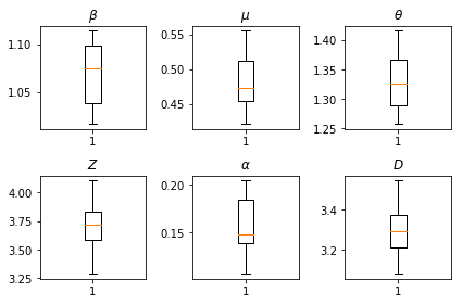
ผลลัพธ์จากการอนุมานของเรา เราวางแผนค่าโอกาสสูงสุดสำหรับทุกพารามิเตอร์ทั่วโลกเพื่อแสดงความเปลี่ยนแปลงของพวกเขาข้ามของเรา num_batches วิ่งอิสระของการอนุมาน ซึ่งสอดคล้องกับตาราง S1 ในเอกสารประกอบ
fig, axs = plt.subplots(2, 3)
axs[0, 0].boxplot(best_parameters.documented_infectious_tx_rate,
                  whis=(2.5,97.5), sym='')
axs[0, 0].set_title(r'$\beta$')

axs[0, 1].boxplot(best_parameters.undocumented_infectious_tx_relative_rate,
                  whis=(2.5,97.5), sym='')
axs[0, 1].set_title(r'$\mu$')

axs[0, 2].boxplot(best_parameters.intercity_underreporting_factor,
                  whis=(2.5,97.5), sym='')
axs[0, 2].set_title(r'$\theta$')

axs[1, 0].boxplot(best_parameters.average_latency_period,
                  whis=(2.5,97.5), sym='')
axs[1, 0].set_title(r'$Z$')

axs[1, 1].boxplot(best_parameters.fraction_of_documented_infections,
                  whis=(2.5,97.5), sym='')
axs[1, 1].set_title(r'$\alpha$')

axs[1, 2].boxplot(best_parameters.average_infection_duration,
                  whis=(2.5,97.5), sym='')
axs[1, 2].set_title(r'$D$')
plt.tight_layout()