
| | |  ดูแหล่งที่มาบน GitHub ดูแหล่งที่มาบน GitHub | |
อาคารออกจากรถที่ทำใน MNIST กวดวิชา, กวดวิชานี้สำรวจผลงานล่าสุดของ Huang et al, ที่แสดงให้เห็นว่าชุดข้อมูลต่างๆ ส่งผลต่อการเปรียบเทียบประสิทธิภาพอย่างไร ในงาน ผู้เขียนพยายามทำความเข้าใจว่าโมเดลแมชชีนเลิร์นนิงแบบคลาสสิกสามารถเรียนรู้ได้อย่างไรและเมื่อใด ตลอดจน (หรือดีกว่า) โมเดลควอนตัม งานนี้ยังแสดงการแยกประสิทธิภาพเชิงประจักษ์ระหว่างโมเดลการเรียนรู้ของเครื่องคลาสสิกและควอนตัมผ่านชุดข้อมูลที่สร้างขึ้นอย่างพิถีพิถัน คุณจะ:
- เตรียมชุดข้อมูล Fashion-MNIST ขนาดลดลง
- ใช้วงจรควอนตัมเพื่อติดป้ายกำกับชุดข้อมูลใหม่และคำนวณฟีเจอร์ Projected Quantum Kernel (PQK)
- ฝึกโครงข่ายประสาทเทียมแบบคลาสสิกบนชุดข้อมูลที่มีการติดป้ายกำกับใหม่ และเปรียบเทียบประสิทธิภาพกับแบบจำลองที่มีสิทธิ์เข้าถึงคุณลักษณะ PQK
ติดตั้ง
pip install tensorflow==2.4.1 tensorflow-quantum
# Update package resources to account for version changes.
import importlib, pkg_resources
importlib.reload(pkg_resources)
import cirq
import sympy
import numpy as np
import tensorflow as tf
import tensorflow_quantum as tfq

# visualization tools
%matplotlib inline
import matplotlib.pyplot as plt
from cirq.contrib.svg import SVGCircuit
np.random.seed(1234)
1. การเตรียมข้อมูล
คุณจะเริ่มต้นด้วยการเตรียมชุดข้อมูล fashion-MNIST สำหรับการรันบนคอมพิวเตอร์ควอนตัม
1.1 ดาวน์โหลดแฟชั่น-MNIST
ขั้นตอนแรกคือการรับชุดข้อมูลผู้เชี่ยวชาญด้านแฟชั่นแบบดั้งเดิม ซึ่งสามารถทำได้โดยใช้ tf.keras.datasets โมดูล
(x_train, y_train), (x_test, y_test) = tf.keras.datasets.fashion_mnist.load_data()

# Rescale the images from [0,255] to the [0.0,1.0] range.
x_train, x_test = x_train/255.0, x_test/255.0

print("Number of original training examples:", len(x_train))
print("Number of original test examples:", len(x_test))
Number of original training examples: 60000
Number of original test examples: 10000
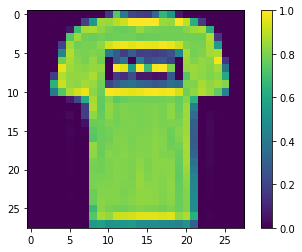
กรองชุดข้อมูลเพื่อเก็บเฉพาะเสื้อยืด/เสื้อและชุดเดรส ลบคลาสอื่นๆ ในเวลาเดียวกันแปลงฉลาก y เพื่อ boolean: True สำหรับ 0 และเท็จ 3
def filter_03(x, y):
    keep = (y == 0) | (y == 3)
    x, y = x[keep], y[keep]
    y = y == 0
    return x,y
x_train, y_train = filter_03(x_train, y_train)
x_test, y_test = filter_03(x_test, y_test)

print("Number of filtered training examples:", len(x_train))
print("Number of filtered test examples:", len(x_test))
Number of filtered training examples: 12000
Number of filtered test examples: 2000
print(y_train[0])

plt.imshow(x_train[0, :, :])
plt.colorbar()
True
<matplotlib.colorbar.Colorbar at 0x7f6db42c3460>
1.2 ลดขนาดภาพ
เช่นเดียวกับตัวอย่าง MNIST คุณจะต้องลดขนาดภาพเหล่านี้เพื่อให้อยู่ภายในขอบเขตสำหรับคอมพิวเตอร์ควอนตัมปัจจุบัน ในเวลานี้อย่างไรก็ตามคุณจะใช้การเปลี่ยนแปลง PCA เพื่อลดขนาดแทน tf.image.resize การดำเนินงาน
def truncate_x(x_train, x_test, n_components=10):
  """Perform PCA on image dataset keeping the top `n_components` components."""
  n_points_train = tf.gather(tf.shape(x_train), 0)
  n_points_test = tf.gather(tf.shape(x_test), 0)

  # Flatten to 1D
  x_train = tf.reshape(x_train, [n_points_train, -1])
  x_test = tf.reshape(x_test, [n_points_test, -1])

  # Normalize.
  feature_mean = tf.reduce_mean(x_train, axis=0)
  x_train_normalized = x_train - feature_mean
  x_test_normalized = x_test - feature_mean

  # Truncate.
  e_values, e_vectors = tf.linalg.eigh(
      tf.einsum('ji,jk->ik', x_train_normalized, x_train_normalized))
  return tf.einsum('ij,jk->ik', x_train_normalized, e_vectors[:,-n_components:]), \
    tf.einsum('ij,jk->ik', x_test_normalized, e_vectors[:, -n_components:])
DATASET_DIM = 10
x_train, x_test = truncate_x(x_train, x_test, n_components=DATASET_DIM)
print(f'New datapoint dimension:', len(x_train[0]))
New datapoint dimension: 10
ขั้นตอนสุดท้ายคือการลดขนาดของชุดข้อมูลให้เหลือเพียงจุดข้อมูลการฝึกอบรม 1,000 จุดและจุดข้อมูลการทดสอบ 200 จุด
N_TRAIN = 1000
N_TEST = 200
x_train, x_test = x_train[:N_TRAIN], x_test[:N_TEST]
y_train, y_test = y_train[:N_TRAIN], y_test[:N_TEST]
print("New number of training examples:", len(x_train))
print("New number of test examples:", len(x_test))
New number of training examples: 1000
New number of test examples: 200
2. การติดฉลากใหม่และคำนวณคุณสมบัติ PQK
ตอนนี้ คุณจะเตรียมชุดข้อมูลควอนตัม "แบบหยั่งเชิง" โดยผสมผสานส่วนประกอบควอนตัมและติดป้ายกำกับชุดข้อมูล fashion-MNIST ที่ถูกตัดทอนใหม่ที่คุณได้สร้างไว้ด้านบน เพื่อให้ได้การแยกความแตกต่างระหว่างวิธีควอนตัมและแบบคลาสสิก ขั้นแรกคุณต้องเตรียมคุณสมบัติ PQK แล้วจึงติดป้ายกำกับเอาต์พุตใหม่ตามค่าของพวกมัน
2.1 การเข้ารหัสควอนตัมและคุณสมบัติ PQK
คุณจะสร้างชุดใหม่ของคุณสมบัติขึ้นอยู่กับ x_train , y_train , x_test และ y_test ที่ถูกกำหนดให้เป็น 1-RDM บน qubits ทั้งหมด:
\(V(x_{\text{train} } / n_{\text{trotter} }) ^ {n_{\text{trotter} } } U_{\text{1qb} } | 0 \rangle\)
ที่ไหน \(U_\text{1qb}\) เป็นกำแพงผลัดคิวบิตเดียวและ \(V(\hat{\theta}) = e^{-i\sum_i \hat{\theta_i} (X_i X_{i+1} + Y_i Y_{i+1} + Z_i Z_{i+1})}\)
ขั้นแรก คุณสามารถสร้างกำแพงของการหมุน qubit เดียว:
def single_qubit_wall(qubits, rotations):
  """Prepare a single qubit X,Y,Z rotation wall on `qubits`."""
  wall_circuit = cirq.Circuit()
  for i, qubit in enumerate(qubits):
    for j, gate in enumerate([cirq.X, cirq.Y, cirq.Z]):
      wall_circuit.append(gate(qubit) ** rotations[i][j])

  return wall_circuit
คุณสามารถตรวจสอบงานนี้ได้อย่างรวดเร็วโดยดูที่วงจร:
SVGCircuit(single_qubit_wall(
    cirq.GridQubit.rect(1,4), np.random.uniform(size=(4, 3))))

ถัดไปคุณสามารถเตรียมความพร้อม \(V(\hat{\theta})\) ด้วยความช่วยเหลือของ tfq.util.exponential ซึ่งสามารถ exponentiate ใดเดินทาง cirq.PauliSum วัตถุ:
def v_theta(qubits):
  """Prepares a circuit that generates V(\theta)."""
  ref_paulis = [
      cirq.X(q0) * cirq.X(q1) + \
      cirq.Y(q0) * cirq.Y(q1) + \
      cirq.Z(q0) * cirq.Z(q1) for q0, q1 in zip(qubits, qubits[1:])
  ]
  exp_symbols = list(sympy.symbols('ref_0:'+str(len(ref_paulis))))
  return tfq.util.exponential(ref_paulis, exp_symbols), exp_symbols
วงจรนี้อาจตรวจสอบได้ยากขึ้นเล็กน้อยโดยดูที่ แต่คุณยังสามารถตรวจสอบกรณีสอง qubit เพื่อดูว่าเกิดอะไรขึ้น:
test_circuit, test_symbols = v_theta(cirq.GridQubit.rect(1, 2))
print(f'Symbols found in circuit:{test_symbols}')
SVGCircuit(test_circuit)
Symbols found in circuit:[ref_0]

ตอนนี้คุณมีหน่วยการสร้างทั้งหมดที่จำเป็นสำหรับการรวมวงจรการเข้ารหัสทั้งหมดเข้าด้วยกัน:
def prepare_pqk_circuits(qubits, classical_source, n_trotter=10):
  """Prepare the pqk feature circuits around a dataset."""
  n_qubits = len(qubits)
  n_points = len(classical_source)

  # Prepare random single qubit rotation wall.
  random_rots = np.random.uniform(-2, 2, size=(n_qubits, 3))
  initial_U = single_qubit_wall(qubits, random_rots)

  # Prepare parametrized V
  V_circuit, symbols = v_theta(qubits)
  exp_circuit = cirq.Circuit(V_circuit for t in range(n_trotter))

  # Convert to `tf.Tensor`
  initial_U_tensor = tfq.convert_to_tensor([initial_U])
  initial_U_splat = tf.tile(initial_U_tensor, [n_points])

  full_circuits = tfq.layers.AddCircuit()(
      initial_U_splat, append=exp_circuit)
  # Replace placeholders in circuits with values from `classical_source`.
  return tfq.resolve_parameters(
      full_circuits, tf.convert_to_tensor([str(x) for x in symbols]),
      tf.convert_to_tensor(classical_source*(n_qubits/3)/n_trotter))
เลือก qubits และเตรียมวงจรการเข้ารหัสข้อมูล:
qubits = cirq.GridQubit.rect(1, DATASET_DIM + 1)
q_x_train_circuits = prepare_pqk_circuits(qubits, x_train)
q_x_test_circuits = prepare_pqk_circuits(qubits, x_test)
ถัดไปคำนวณ PQK คุณสมบัติขึ้นอยู่กับ 1 RDM ของวงจรชุดข้อมูลข้างต้นและเก็บผลใน rdm เป็น tf.Tensor มีรูปร่าง [n_points, n_qubits, 3] รายการใน rdm[i][j][k] = \(\langle \psi_i | OP^k_j | \psi_i \rangle\) ที่ i ดัชนีมากกว่า datapoints, j ดัชนีมากกว่า qubits และ k ดัชนีมากกว่า \(\lbrace \hat{X}, \hat{Y}, \hat{Z} \rbrace\)
def get_pqk_features(qubits, data_batch):
  """Get PQK features based on above construction."""
  ops = [[cirq.X(q), cirq.Y(q), cirq.Z(q)] for q in qubits]
  ops_tensor = tf.expand_dims(tf.reshape(tfq.convert_to_tensor(ops), -1), 0)
  batch_dim = tf.gather(tf.shape(data_batch), 0)
  ops_splat = tf.tile(ops_tensor, [batch_dim, 1])
  exp_vals = tfq.layers.Expectation()(data_batch, operators=ops_splat)
  rdm = tf.reshape(exp_vals, [batch_dim, len(qubits), -1])
  return rdm
x_train_pqk = get_pqk_features(qubits, q_x_train_circuits)
x_test_pqk = get_pqk_features(qubits, q_x_test_circuits)
print('New PQK training dataset has shape:', x_train_pqk.shape)
print('New PQK testing dataset has shape:', x_test_pqk.shape)
New PQK training dataset has shape: (1000, 11, 3)
New PQK testing dataset has shape: (200, 11, 3)
2.2 การติดฉลากใหม่ตามคุณสมบัติ PQK
ตอนนี้คุณมีคุณสมบัติที่ควอนตัมที่สร้างเหล่านี้ใน x_train_pqk และ x_test_pqk มันเป็นเวลาที่จะใหม่ป้ายชุดข้อมูล เพื่อให้เกิดการแยกสูงสุดระหว่างควอนตัมและประสิทธิภาพคลาสสิกที่คุณสามารถ re-label ชุดข้อมูลที่อยู่บนพื้นฐานของข้อมูลสเปกตรัมที่พบใน x_train_pqk และ x_test_pqk
def compute_kernel_matrix(vecs, gamma):
  """Computes d[i][j] = e^ -gamma * (vecs[i] - vecs[j]) ** 2 """
  scaled_gamma = gamma / (
      tf.cast(tf.gather(tf.shape(vecs), 1), tf.float32) * tf.math.reduce_std(vecs))
  return scaled_gamma * tf.einsum('ijk->ij',(vecs[:,None,:] - vecs) ** 2)

def get_spectrum(datapoints, gamma=1.0):
  """Compute the eigenvalues and eigenvectors of the kernel of datapoints."""
  KC_qs = compute_kernel_matrix(datapoints, gamma)
  S, V = tf.linalg.eigh(KC_qs)
  S = tf.math.abs(S)
  return S, V
S_pqk, V_pqk = get_spectrum(
    tf.reshape(tf.concat([x_train_pqk, x_test_pqk], 0), [-1, len(qubits) * 3]))

S_original, V_original = get_spectrum(
    tf.cast(tf.concat([x_train, x_test], 0), tf.float32), gamma=0.005)

print('Eigenvectors of pqk kernel matrix:', V_pqk)
print('Eigenvectors of original kernel matrix:', V_original)
Eigenvectors of pqk kernel matrix: tf.Tensor(
[[-2.09569391e-02  1.05973557e-02  2.16634180e-02 ...  2.80352887e-02
   1.55521873e-02  2.82677952e-02]
 [-2.29303762e-02  4.66355234e-02  7.91163836e-03 ... -6.14174758e-04
  -7.07804322e-01  2.85902526e-02]
 [-1.77853629e-02 -3.00758495e-03 -2.55225878e-02 ... -2.40783971e-02
   2.11018627e-03  2.69009806e-02]
 ...
 [ 6.05797209e-02  1.32483775e-02  2.69536003e-02 ... -1.38843581e-02
   3.05043962e-02  3.85345481e-02]
 [ 6.33309558e-02 -3.04112374e-03  9.77444276e-03 ...  7.48321265e-02
   3.42793856e-03  3.67484428e-02]
 [ 5.86028099e-02  5.84433973e-03  2.64811981e-03 ...  2.82612257e-02
  -3.80136147e-02  3.29943895e-02]], shape=(1200, 1200), dtype=float32)
Eigenvectors of original kernel matrix: tf.Tensor(
[[ 0.03835681  0.0283473  -0.01169789 ...  0.02343717  0.0211248
   0.03206972]
 [-0.04018159  0.00888097 -0.01388255 ...  0.00582427  0.717551
   0.02881948]
 [-0.0166719   0.01350376 -0.03663862 ...  0.02467175 -0.00415936
   0.02195409]
 ...
 [-0.03015648 -0.01671632 -0.01603392 ...  0.00100583 -0.00261221
   0.02365689]
 [ 0.0039777  -0.04998879 -0.00528336 ...  0.01560401 -0.04330755
   0.02782002]
 [-0.01665728 -0.00818616 -0.0432341  ...  0.00088256  0.00927396
   0.01875088]], shape=(1200, 1200), dtype=float32)
ตอนนี้ คุณมีทุกสิ่งที่จำเป็นสำหรับการติดป้ายกำกับชุดข้อมูลอีกครั้ง! ตอนนี้คุณสามารถปรึกษากับผังงานเพื่อทำความเข้าใจวิธีการแยกประสิทธิภาพสูงสุดเมื่อทำการติดฉลากชุดข้อมูลใหม่:
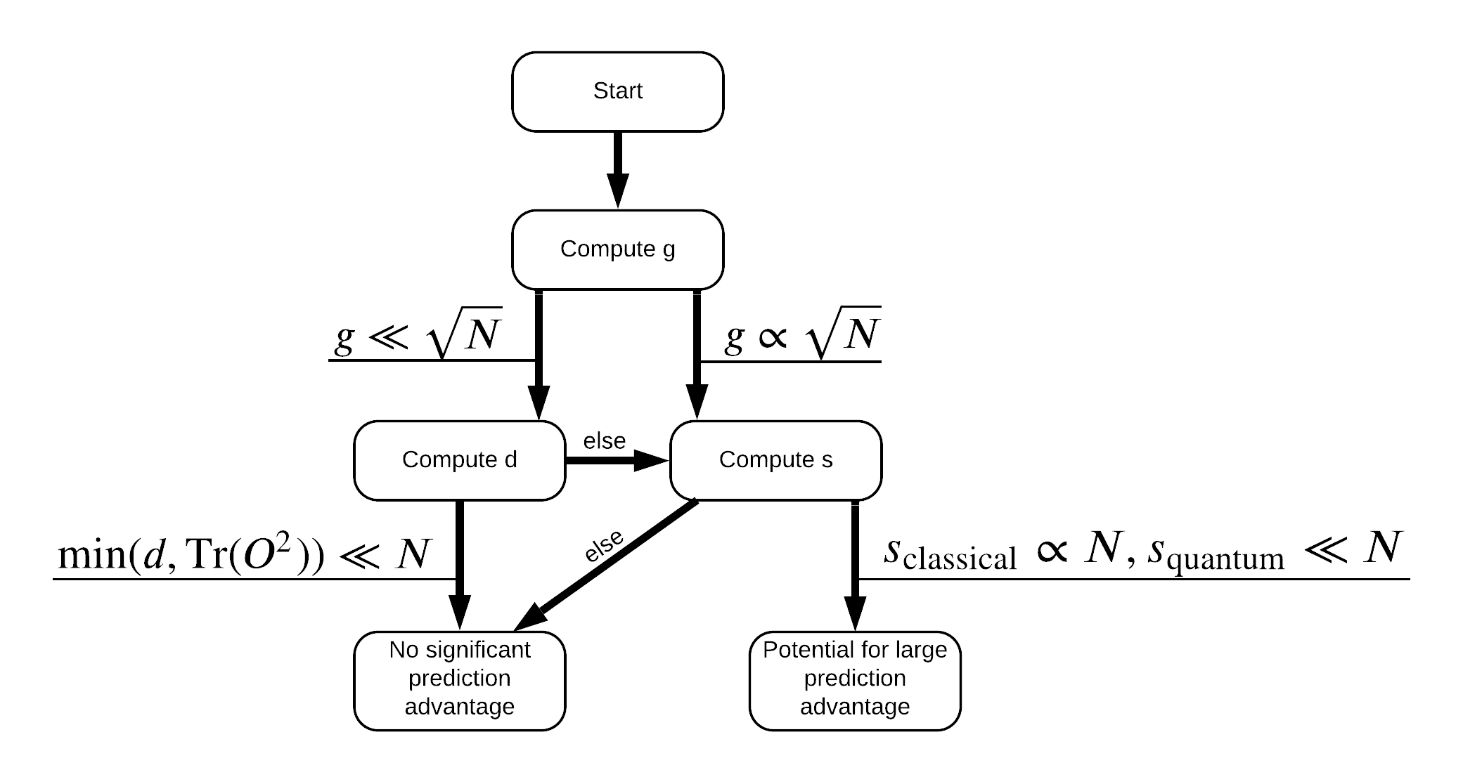
เพื่อเพิ่มการแยกระหว่างควอนตัมและรูปแบบคลาสสิกที่คุณจะพยายามที่จะเพิ่มความแตกต่างของรูปทรงเรขาคณิตระหว่างชุดข้อมูลเดิมและ PQK มีเคอร์เนลเมทริกซ์ \(g(K_1 || K_2) = \sqrt{ || \sqrt{K_2} K_1^{-1} \sqrt{K_2} || _\infty}\) ใช้ S_pqk, V_pqk และ S_original, V_original ค่ามาก \(g\) เพื่อให้แน่ใจว่าคุณเริ่มย้ายไปทางขวาในผังลงไปสู่ความได้เปรียบในการคาดการณ์ในกรณีที่ควอนตัม
def get_stilted_dataset(S, V, S_2, V_2, lambdav=1.1):
  """Prepare new labels that maximize geometric distance between kernels."""
  S_diag = tf.linalg.diag(S ** 0.5)
  S_2_diag = tf.linalg.diag(S_2 / (S_2 + lambdav) ** 2)
  scaling = S_diag @ tf.transpose(V) @ \
            V_2 @ S_2_diag @ tf.transpose(V_2) @ \
            V @ S_diag

  # Generate new lables using the largest eigenvector.
  _, vecs = tf.linalg.eig(scaling)
  new_labels = tf.math.real(
      tf.einsum('ij,j->i', tf.cast(V @ S_diag, tf.complex64), vecs[-1])).numpy()
  # Create new labels and add some small amount of noise.
  final_y = new_labels > np.median(new_labels)
  noisy_y = (final_y ^ (np.random.uniform(size=final_y.shape) > 0.95))
  return noisy_y
y_relabel = get_stilted_dataset(S_pqk, V_pqk, S_original, V_original)
y_train_new, y_test_new = y_relabel[:N_TRAIN], y_relabel[N_TRAIN:]
3. เปรียบเทียบรุ่น
เมื่อคุณได้เตรียมชุดข้อมูลของคุณแล้ว ก็ถึงเวลาเปรียบเทียบประสิทธิภาพของแบบจำลอง คุณจะสร้างเครือข่ายประสาทสองคราทขนาดเล็กและเปรียบเทียบประสิทธิภาพเมื่อพวกเขาจะได้รับการเข้าถึง PQK คุณลักษณะที่พบใน x_train_pqk
3.1 สร้างแบบจำลองที่ปรับปรุง PQK
โดยใช้มาตรฐาน tf.keras คุณลักษณะห้องสมุดตอนนี้คุณสามารถสร้างและรถไฟรูปแบบในการ x_train_pqk และ y_train_new datapoints:
#docs_infra: no_execute
def create_pqk_model():
    model = tf.keras.Sequential()
    model.add(tf.keras.layers.Dense(32, activation='sigmoid', input_shape=[len(qubits) * 3,]))
    model.add(tf.keras.layers.Dense(16, activation='sigmoid'))
    model.add(tf.keras.layers.Dense(1))
    return model

pqk_model = create_pqk_model()
pqk_model.compile(loss=tf.keras.losses.BinaryCrossentropy(from_logits=True),
              optimizer=tf.keras.optimizers.Adam(learning_rate=0.003),
              metrics=['accuracy'])

pqk_model.summary()
Model: "sequential"
_________________________________________________________________
Layer (type)                 Output Shape              Param #
=================================================================
dense (Dense)                (None, 32)                1088
_________________________________________________________________
dense_1 (Dense)              (None, 16)                528
_________________________________________________________________
dense_2 (Dense)              (None, 1)                 17
=================================================================
Total params: 1,633
Trainable params: 1,633
Non-trainable params: 0
_________________________________________________________________
#docs_infra: no_execute
pqk_history = pqk_model.fit(tf.reshape(x_train_pqk, [N_TRAIN, -1]),
          y_train_new,
          batch_size=32,
          epochs=1000,
          verbose=0,
          validation_data=(tf.reshape(x_test_pqk, [N_TEST, -1]), y_test_new))
3.2 สร้างแบบจำลองคลาสสิก
คล้ายกับโค้ดด้านบน คุณสามารถสร้างโมเดลคลาสสิกที่ไม่สามารถเข้าถึงคุณลักษณะ PQK ในชุดข้อมูลแบบเอียงได้ รุ่นนี้สามารถรับการฝึกอบรมโดยใช้ x_train และ y_label_new
#docs_infra: no_execute
def create_fair_classical_model():
    model = tf.keras.Sequential()
    model.add(tf.keras.layers.Dense(32, activation='sigmoid', input_shape=[DATASET_DIM,]))
    model.add(tf.keras.layers.Dense(16, activation='sigmoid'))
    model.add(tf.keras.layers.Dense(1))
    return model

model = create_fair_classical_model()
model.compile(loss=tf.keras.losses.BinaryCrossentropy(from_logits=True),
              optimizer=tf.keras.optimizers.Adam(learning_rate=0.03),
              metrics=['accuracy'])

model.summary()
Model: "sequential_1"
_________________________________________________________________
Layer (type)                 Output Shape              Param #
=================================================================
dense_3 (Dense)              (None, 32)                352
_________________________________________________________________
dense_4 (Dense)              (None, 16)                528
_________________________________________________________________
dense_5 (Dense)              (None, 1)                 17
=================================================================
Total params: 897
Trainable params: 897
Non-trainable params: 0
_________________________________________________________________
#docs_infra: no_execute
classical_history = model.fit(x_train,
          y_train_new,
          batch_size=32,
          epochs=1000,
          verbose=0,
          validation_data=(x_test, y_test_new))
3.3 เปรียบเทียบประสิทธิภาพ
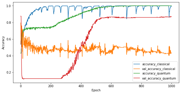
ตอนนี้ คุณได้ฝึกโมเดลทั้งสองแล้ว คุณสามารถพล็อตช่องว่างด้านประสิทธิภาพในข้อมูลการตรวจสอบความถูกต้องระหว่างทั้งสองได้อย่างรวดเร็ว โดยทั่วไปแล้วทั้งสองรุ่นจะมีความแม่นยำ > 0.9 ในข้อมูลการฝึก อย่างไรก็ตาม จากข้อมูลการตรวจสอบความถูกต้อง เป็นที่ชัดเจนว่ามีเพียงข้อมูลที่พบในคุณลักษณะ PQK เท่านั้นที่เพียงพอที่จะทำให้แบบจำลองนี้เป็นภาพรวมได้ดีสำหรับอินสแตนซ์ที่มองไม่เห็น
#docs_infra: no_execute
plt.figure(figsize=(10,5))
plt.plot(classical_history.history['accuracy'], label='accuracy_classical')
plt.plot(classical_history.history['val_accuracy'], label='val_accuracy_classical')
plt.plot(pqk_history.history['accuracy'], label='accuracy_quantum')
plt.plot(pqk_history.history['val_accuracy'], label='val_accuracy_quantum')
plt.xlabel('Epoch')
plt.ylabel('Accuracy')
plt.legend()
<matplotlib.legend.Legend at 0x7f6d846ecee0>
4. ข้อสรุปที่สำคัญ
มีข้อสรุปที่สำคัญหลายประการที่คุณสามารถวาดจากนี้และมี MNIST ทดลอง:
ไม่น่าเป็นไปได้มากที่โมเดลควอนตัมในปัจจุบันจะเอาชนะประสิทธิภาพของโมเดลคลาสสิกกับข้อมูลคลาสสิกได้ โดยเฉพาะชุดข้อมูลคลาสสิกในปัจจุบันที่สามารถมีจุดข้อมูลได้มากกว่าหนึ่งล้านจุด
เพียงเพราะข้อมูลอาจมาจากวงจรควอนตัมที่จำลองแบบยากไปจนถึงแบบคลาสสิก ไม่จำเป็นต้องทำให้ข้อมูลเรียนรู้ได้ยากสำหรับแบบจำลองคลาสสิก
ชุดข้อมูล (ในท้ายที่สุดมีลักษณะเป็นควอนตัม) ที่ง่ายสำหรับโมเดลควอนตัมในการเรียนรู้ และยากสำหรับโมเดลคลาสสิกที่จะเรียนรู้มีอยู่ โดยไม่คำนึงถึงสถาปัตยกรรมแบบจำลองหรืออัลกอริธึมการฝึกอบรมที่ใช้