
| | |  ดูแหล่งที่มาบน GitHub ดูแหล่งที่มาบน GitHub | |
TensorFlow Quantum นำควอนตัมดั้งเดิมมาสู่ระบบนิเวศ TensorFlow ตอนนี้นักวิจัยควอนตัมสามารถใช้เครื่องมือจาก TensorFlow ได้แล้ว ในบทช่วยสอนนี้ คุณจะเจาะลึกถึงการผสมผสาน TensorBoard เข้ากับการวิจัยคอมพิวเตอร์ควอนตัมของคุณ การใช้ บทช่วยสอน DCGAN จาก TensorFlow คุณจะสามารถสร้างการทดลองและการสร้างภาพข้อมูลได้อย่างรวดเร็วคล้ายกับที่ทำโดย Niu et al . พูดกว้างๆ คุณจะ:
- ฝึก GAN เพื่อผลิตตัวอย่างที่ดูเหมือนมาจากวงจรควอนตัม
- เห็นภาพความคืบหน้าของการฝึกอบรมตลอดจนวิวัฒนาการการจัดจำหน่ายเมื่อเวลาผ่านไป
- เปรียบเทียบการทดสอบโดยสำรวจกราฟการคำนวณ
pip install tensorflow==2.7.0 tensorflow-quantum tensorboard_plugin_profile==2.4.0
# Update package resources to account for version changes.
import importlib, pkg_resources
importlib.reload(pkg_resources)
<module 'pkg_resources' from '/tmpfs/src/tf_docs_env/lib/python3.7/site-packages/pkg_resources/__init__.py'>
#docs_infra: no_execute
%load_ext tensorboard
import datetime
import time
import cirq
import tensorflow as tf
import tensorflow_quantum as tfq
from tensorflow.keras import layers

# visualization tools
%matplotlib inline
import matplotlib.pyplot as plt
from cirq.contrib.svg import SVGCircuit
2022-02-04 12:46:52.770534: E tensorflow/stream_executor/cuda/cuda_driver.cc:271] failed call to cuInit: CUDA_ERROR_NO_DEVICE: no CUDA-capable device is detected
1. การสร้างข้อมูล
เริ่มต้นด้วยการรวบรวมข้อมูล คุณสามารถใช้ TensorFlow Quantum เพื่อสร้างตัวอย่างบิตสตริงได้อย่างรวดเร็ว ซึ่งจะเป็นแหล่งข้อมูลหลักสำหรับการทดสอบที่เหลือของคุณ เช่นเดียวกับ Niu และคณะ คุณจะได้สำรวจว่าการจำลองการสุ่มตัวอย่างจากวงจรสุ่มที่มีความลึกลดลงอย่างมากนั้นง่ายเพียงใด ขั้นแรกให้กำหนดผู้ช่วยบางคน:
def generate_circuit(qubits):
    """Generate a random circuit on qubits."""
    random_circuit = cirq.generate_boixo_2018_supremacy_circuits_v2(
        qubits, cz_depth=2, seed=1234)
    return random_circuit

def generate_data(circuit, n_samples):
    """Draw n_samples samples from circuit into a tf.Tensor."""
    return tf.squeeze(tfq.layers.Sample()(circuit, repetitions=n_samples).to_tensor())
ตอนนี้คุณสามารถตรวจสอบวงจรและข้อมูลตัวอย่างบางส่วนได้:
qubits = cirq.GridQubit.rect(1, 5)
random_circuit_m = generate_circuit(qubits) + cirq.measure_each(*qubits)
SVGCircuit(random_circuit_m)
findfont: Font family ['Arial'] not found. Falling back to DejaVu Sans.

samples = cirq.sample(random_circuit_m, repetitions=10)
print('10 Random bitstrings from this circuit:')
print(samples)
10 Random bitstrings from this circuit:
(0, 0)=1000001000
(0, 1)=0000001010
(0, 2)=1010000100
(0, 3)=0010000110
(0, 4)=0110110010
คุณสามารถทำสิ่งเดียวกันใน TensorFlow Quantum ด้วย:
generate_data(random_circuit_m, 10)
<tf.Tensor: shape=(10, 5), dtype=int8, numpy=
array([[0, 0, 0, 0, 0],
       [0, 0, 0, 0, 0],
       [0, 0, 1, 0, 0],
       [0, 1, 0, 0, 0],
       [0, 1, 0, 0, 0],
       [0, 1, 1, 0, 0],
       [1, 0, 0, 0, 0],
       [1, 0, 0, 1, 0],
       [1, 1, 1, 0, 0],
       [1, 1, 1, 0, 0]], dtype=int8)>
ตอนนี้คุณสามารถสร้างข้อมูลการฝึกอบรมของคุณได้อย่างรวดเร็วด้วย:
N_SAMPLES = 60000
N_QUBITS = 10
QUBITS = cirq.GridQubit.rect(1, N_QUBITS)
REFERENCE_CIRCUIT = generate_circuit(QUBITS)
all_data = generate_data(REFERENCE_CIRCUIT, N_SAMPLES)
all_data
<tf.Tensor: shape=(60000, 10), dtype=int8, numpy=
array([[0, 0, 0, ..., 0, 0, 0],
       [0, 0, 0, ..., 0, 0, 0],
       [0, 0, 0, ..., 0, 0, 0],
       ...,
       [1, 1, 1, ..., 1, 1, 1],
       [1, 1, 1, ..., 1, 1, 1],
       [1, 1, 1, ..., 1, 1, 1]], dtype=int8)>
จะเป็นประโยชน์ในการกำหนดฟังก์ชันตัวช่วยบางอย่างเพื่อให้เห็นภาพเมื่อการฝึกอบรมกำลังดำเนินไป ปริมาณที่น่าสนใจที่จะใช้คือ:
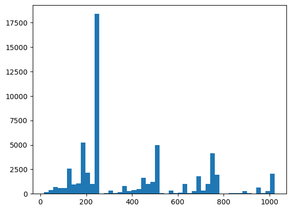
- ค่าจำนวนเต็มของกลุ่มตัวอย่าง เพื่อให้คุณสามารถสร้างฮิสโตแกรมของการแจกแจงได้
- ค่าประมาณความเที่ยงตรงของ XEB เชิงเส้น ของชุดตัวอย่าง เพื่อบ่งชี้ว่าตัวอย่างมี "สุ่มควอนตัมอย่างแท้จริง" อย่างไร
@tf.function
def bits_to_ints(bits):
    """Convert tensor of bitstrings to tensor of ints."""
    sigs = tf.constant([1 << i for i in range(N_QUBITS)], dtype=tf.int32)
    rounded_bits = tf.clip_by_value(tf.math.round(
        tf.cast(bits, dtype=tf.dtypes.float32)), clip_value_min=0, clip_value_max=1)
    return tf.einsum('jk,k->j', tf.cast(rounded_bits, dtype=tf.dtypes.int32), sigs)

@tf.function
def xeb_fid(bits):
    """Compute linear XEB fidelity of bitstrings."""
    final_probs = tf.squeeze(
        tf.abs(tfq.layers.State()(REFERENCE_CIRCUIT).to_tensor()) ** 2)
    nums = bits_to_ints(bits)
    return (2 ** N_QUBITS) * tf.reduce_mean(tf.gather(final_probs, nums)) - 1.0
ที่นี่คุณสามารถเห็นภาพการแจกจ่ายและการตรวจสอบสุขภาพจิตโดยใช้ XEB:
plt.hist(bits_to_ints(all_data).numpy(), 50)
plt.show()
xeb_fid(all_data)
<tf.Tensor: shape=(), dtype=float32, numpy=-0.0015467405>
2. สร้างแบบจำลอง
คุณสามารถใช้ส่วนประกอบที่เกี่ยวข้องจาก บทช่วยสอน DCGAN สำหรับกรณีควอนตัมได้ที่นี่ แทนที่จะสร้างตัวเลข MNIST GAN ใหม่จะถูกใช้เพื่อสร้างตัวอย่างบิตสตริงที่มีความยาว N_QUBITS
LATENT_DIM = 100
def make_generator_model():
    """Construct generator model."""
    model = tf.keras.Sequential()
    model.add(layers.Dense(256, use_bias=False, input_shape=(LATENT_DIM,)))
    model.add(layers.Dense(128, activation='relu'))
    model.add(layers.Dropout(0.3))
    model.add(layers.Dense(64, activation='relu'))
    model.add(layers.Dense(N_QUBITS, activation='relu'))

    return model

def make_discriminator_model():
    """Constrcut discriminator model."""
    model = tf.keras.Sequential()
    model.add(layers.Dense(256, use_bias=False, input_shape=(N_QUBITS,)))
    model.add(layers.Dense(128, activation='relu'))
    model.add(layers.Dropout(0.3))
    model.add(layers.Dense(32, activation='relu'))
    model.add(layers.Dense(1))

    return model
ถัดไป สร้างตัวอย่างโมเดลเครื่องกำเนิดไฟฟ้าและตัวแบ่งแยก กำหนดความสูญเสีย และสร้างฟังก์ชัน train_step เพื่อใช้สำหรับลูปการฝึกหลักของคุณ:
discriminator = make_discriminator_model()
generator = make_generator_model()
cross_entropy = tf.keras.losses.BinaryCrossentropy(from_logits=True)
def discriminator_loss(real_output, fake_output):
    """Compute discriminator loss."""
    real_loss = cross_entropy(tf.ones_like(real_output), real_output)
    fake_loss = cross_entropy(tf.zeros_like(fake_output), fake_output)
    total_loss = real_loss + fake_loss
    return total_loss

def generator_loss(fake_output):
    """Compute generator loss."""
    return cross_entropy(tf.ones_like(fake_output), fake_output)

generator_optimizer = tf.keras.optimizers.Adam(1e-4)
discriminator_optimizer = tf.keras.optimizers.Adam(1e-4)
BATCH_SIZE=256

@tf.function
def train_step(images):
    """Run train step on provided image batch."""
    noise = tf.random.normal([BATCH_SIZE, LATENT_DIM])
    with tf.GradientTape() as gen_tape, tf.GradientTape() as disc_tape:
        generated_images = generator(noise, training=True)

        real_output = discriminator(images, training=True)
        fake_output = discriminator(generated_images, training=True)

        gen_loss = generator_loss(fake_output)
        disc_loss = discriminator_loss(real_output, fake_output)

    gradients_of_generator = gen_tape.gradient(
        gen_loss, generator.trainable_variables)
    gradients_of_discriminator = disc_tape.gradient(
        disc_loss, discriminator.trainable_variables)

    generator_optimizer.apply_gradients(
        zip(gradients_of_generator, generator.trainable_variables))
    discriminator_optimizer.apply_gradients(
        zip(gradients_of_discriminator, discriminator.trainable_variables))

    return gen_loss, disc_loss
ตอนนี้ คุณมีส่วนประกอบทั้งหมดที่จำเป็นสำหรับโมเดลของคุณแล้ว คุณสามารถตั้งค่าฟังก์ชันการฝึกที่รวมการแสดงภาพ TensorBoard ไว้ด้วย ขั้นแรกให้ตั้งค่าตัวเขียนไฟล์ TensorBoard:
logdir = "tb_logs/" + datetime.datetime.now().strftime("%Y%m%d-%H%M%S")
file_writer = tf.summary.create_file_writer(logdir + "/metrics")
file_writer.set_as_default()
เมื่อใช้โมดูล tf.summary คุณสามารถรวมการบันทึก scalar histogram (รวมถึงอื่นๆ) เข้ากับ TensorBoard ภายในฟังก์ชัน train หลักได้:
def train(dataset, epochs, start_epoch=1):
    """Launch full training run for the given number of epochs."""
    # Log original training distribution.
    tf.summary.histogram('Training Distribution', data=bits_to_ints(dataset), step=0)

    batched_data = tf.data.Dataset.from_tensor_slices(dataset).shuffle(N_SAMPLES).batch(512)
    t = time.time()
    for epoch in range(start_epoch, start_epoch + epochs):
        for i, image_batch in enumerate(batched_data):
            # Log batch-wise loss.
            gl, dl = train_step(image_batch)
            tf.summary.scalar(
                'Generator loss', data=gl, step=epoch * len(batched_data) + i)
            tf.summary.scalar(
                'Discriminator loss', data=dl, step=epoch * len(batched_data) + i)

        # Log full dataset XEB Fidelity and generated distribution.
        generated_samples = generator(tf.random.normal([N_SAMPLES, 100]))
        tf.summary.scalar(
        'Generator XEB Fidelity Estimate', data=xeb_fid(generated_samples), step=epoch)
        tf.summary.histogram(
        'Generator distribution', data=bits_to_ints(generated_samples), step=epoch)
        # Log new samples drawn from this particular random circuit.
        random_new_distribution = generate_data(REFERENCE_CIRCUIT, N_SAMPLES)
        tf.summary.histogram(
        'New round of True samples', data=bits_to_ints(random_new_distribution), step=epoch)

        if epoch % 10 == 0:
            print('Epoch {}, took {}(s)'.format(epoch, time.time() - t))
            t = time.time()
3. Vizualize การฝึกอบรมและประสิทธิภาพ
แดชบอร์ด TensorBoard สามารถเปิดใช้งานได้ด้วย:
#docs_infra: no_execute
%tensorboard --logdir tb_logs/
เมื่อโทรเรียก train แดชบอร์ด TensoBoard จะอัปเดตอัตโนมัติพร้อมสถิติสรุปทั้งหมดที่ระบุในลูปการฝึก
train(all_data, epochs=50)
Epoch 10, took 9.325464487075806(s)
Epoch 20, took 7.684147119522095(s)
Epoch 30, took 7.508770704269409(s)
Epoch 40, took 7.5157341957092285(s)
Epoch 50, took 7.533370494842529(s)
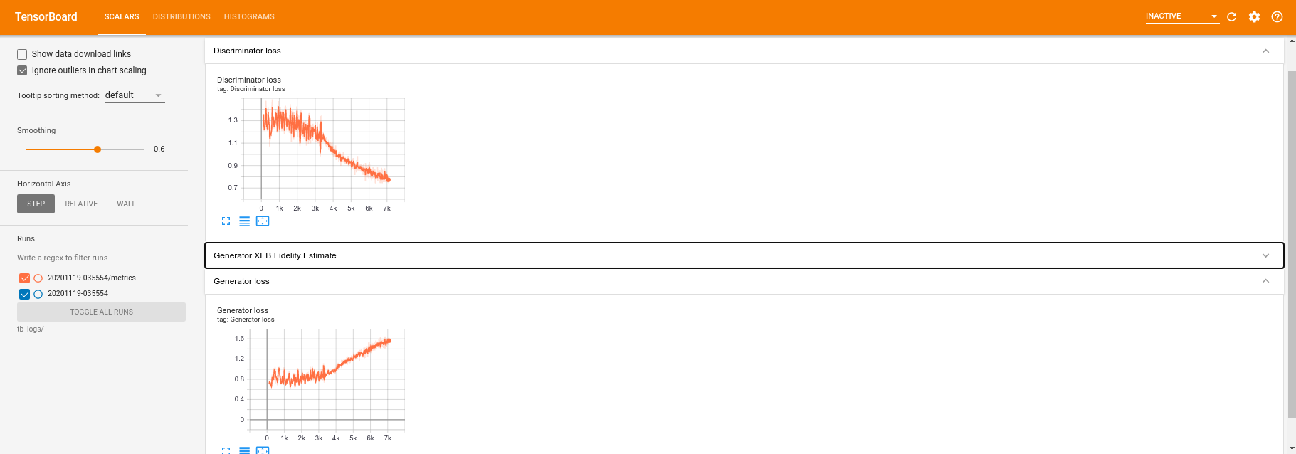
ในขณะที่การฝึกอบรมกำลังทำงาน (และเมื่อเสร็จสิ้น) คุณสามารถตรวจสอบปริมาณสเกลาร์ได้:
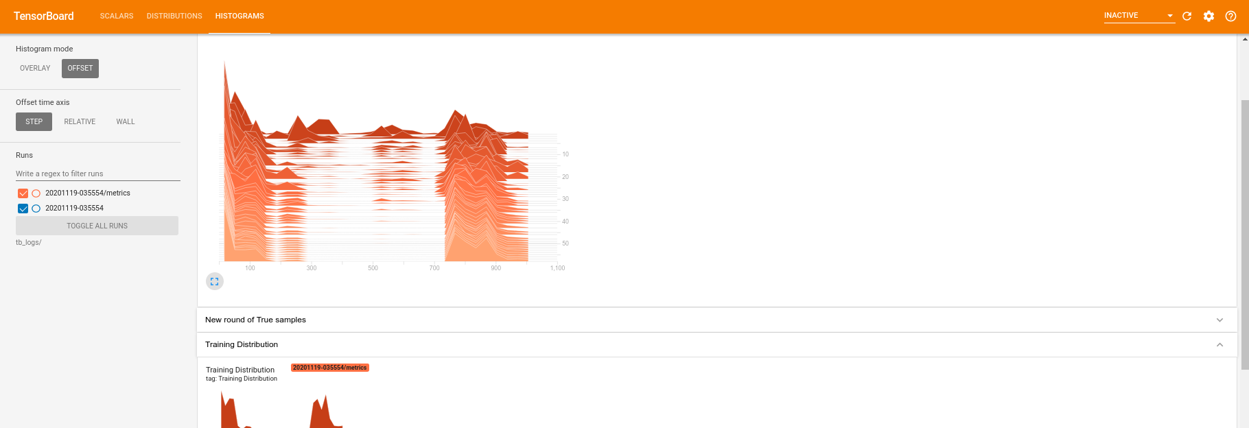
การสลับไปที่แท็บฮิสโตแกรม คุณยังสามารถดูว่าเครือข่ายตัวสร้างสร้างตัวอย่างจากการแจกแจงควอนตัมได้ดีเพียงใด:
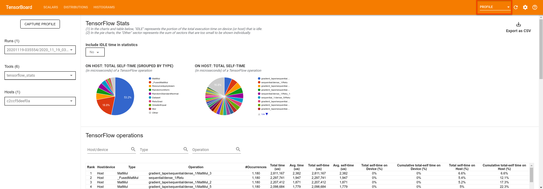
นอกเหนือจากการตรวจสอบสถิติสรุปที่เกี่ยวข้องกับการทดสอบของคุณแบบเรียลไทม์แล้ว TensorBoard ยังสามารถช่วยคุณกำหนดโปรไฟล์การทดสอบของคุณเพื่อระบุปัญหาคอขวดด้านประสิทธิภาพ ในการรันโมเดลของคุณอีกครั้งด้วยการตรวจสอบประสิทธิภาพ คุณสามารถทำได้:
tf.profiler.experimental.start(logdir)
train(all_data, epochs=10, start_epoch=50)
tf.profiler.experimental.stop()
Epoch 50, took 0.8879530429840088(s)
TensorBoard จะสร้างโปรไฟล์ของรหัสทั้งหมดระหว่าง tf.profiler.experimental.start และ tf.profiler.experimental.stop ข้อมูลโปรไฟล์นี้สามารถดูได้ในหน้า profile ของ TensorBoard:
ลองเพิ่มความลึกหรือทดลองกับวงจรควอนตัมประเภทต่างๆ ตรวจสอบคุณสมบัติที่ยอดเยี่ยมอื่นๆ ทั้งหมดของ TensorBoard เช่น การปรับแต่ง ไฮเปอร์พารามิเตอร์ที่คุณสามารถรวมเข้ากับการทดลอง TensorFlow Quantum ของคุณ