
 GitHub에서 보기 GitHub에서 보기 |
이번 튜토리얼에서는 딥 러닝을 사용하여 원하는 이미지를 다른 스타일의 이미지로 구성하는 법을 배워보겠습니다(피카소나 반 고흐처럼 그리기를 희망하나요?). 이 기법은 Neural Style Transfer로 알려져 있으며, Leon A. Gatys의 논문 A Neural Algorithm of Artistic Style에 잘 기술되어 있습니다.
참고: 이 튜토리얼은 원래 스타일 전송 알고리즘을 보여줍니다. 이는 이미지 콘텐츠를 특정 스타일로 최적화합니다. 최근의 접근 방식에서는 스타일화된 이미지를 직접 생성하도록 모델을 훈련합니다(CycleGAN과 유사). 이 접근 방식은 훨씬 빠릅니다(최대 1000배).
TensorFlow Hub에서 사전 훈련된 모델을 사용하여 스타일 전송을 간단하게 적용하려면 임의 이미지 스타일화 모델을 사용하는 임의 스타일에 대한 빠른 스타일 전송 튜토리얼을 참조하세요. TensorFlow Lite를 사용한 스타일 전송의 예는 TensorFlow Lite를 사용한 예술적 스타일 전송을 참조하세요.
신경 스타일 전송은 콘텐츠 이미지와 스타일 참조 이미지(유명 화가의 작품 등)라는 두 개의 이미지를 가져와서 출력 이미지가 콘텐츠 이미지처럼 보이지만 스타일 참조 이미지의 스타일로 "페인트"되도록 함께 혼합하는 데 사용되는 최적화 기술입니다.
이는 콘텐츠 이미지의 콘텐츠 통계와 스타일 참조 이미지의 스타일 통계가 일치하도록 출력 이미지를 최적화하여 구현됩니다. 이러한 통계는 컨볼루셔널 네트워크를 사용하여 이미지에서 추출됩니다.
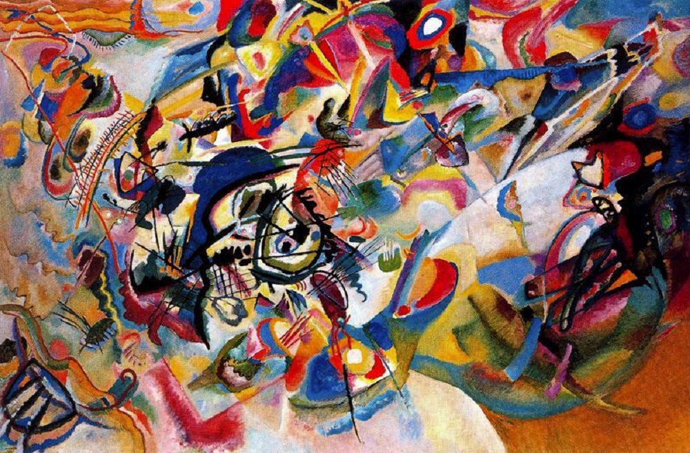
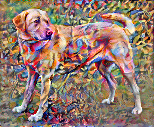
예를 들어, 이 개와 Wassily Kandinsky의 Composition 7의 이미지를 살펴보겠습니다.
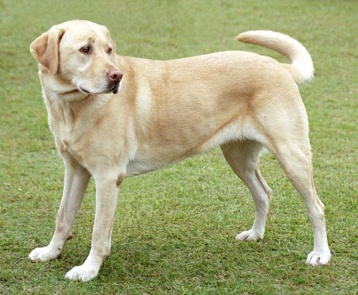
(Yellow Labrador Looking, 출처: Wikimedia Commons, 저자: Elf. 라이선스: CC BY-SA 3.0)
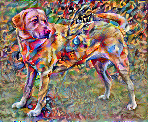
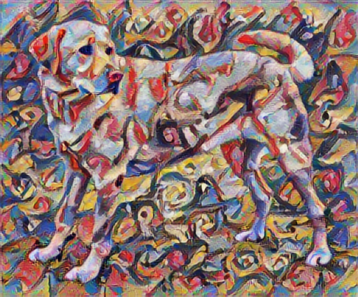
이제 Kandinsky가 이 스타일로만 이 개의 그림을 그리기로 결정했다면 어떤 모습이 될까요? 이렇지 않을까요?
설정
모듈 구성 및 임포트
import os
import tensorflow as tf
# Load compressed models from tensorflow_hub
os.environ['TFHUB_MODEL_LOAD_FORMAT'] = 'COMPRESSED'
2022-12-15 01:04:03.991525: W tensorflow/compiler/xla/stream_executor/platform/default/dso_loader.cc:64] Could not load dynamic library 'libnvinfer.so.7'; dlerror: libnvinfer.so.7: cannot open shared object file: No such file or directory
2022-12-15 01:04:03.991631: W tensorflow/compiler/xla/stream_executor/platform/default/dso_loader.cc:64] Could not load dynamic library 'libnvinfer_plugin.so.7'; dlerror: libnvinfer_plugin.so.7: cannot open shared object file: No such file or directory
2022-12-15 01:04:03.991641: W tensorflow/compiler/tf2tensorrt/utils/py_utils.cc:38] TF-TRT Warning: Cannot dlopen some TensorRT libraries. If you would like to use Nvidia GPU with TensorRT, please make sure the missing libraries mentioned above are installed properly.
import IPython.display as display

import matplotlib.pyplot as plt
import matplotlib as mpl
mpl.rcParams['figure.figsize'] = (12, 12)
mpl.rcParams['axes.grid'] = False

import numpy as np
import PIL.Image
import time
import functools
def tensor_to_image(tensor):
  tensor = tensor*255
  tensor = np.array(tensor, dtype=np.uint8)
  if np.ndim(tensor)>3:
    assert tensor.shape[0] == 1
    tensor = tensor[0]
  return PIL.Image.fromarray(tensor)
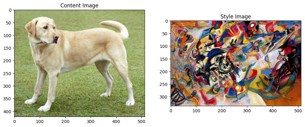
이미지를 다운로드받고 스타일 참조 이미지와 콘텐츠 이미지를 선택합니다:
content_path = tf.keras.utils.get_file('YellowLabradorLooking_new.jpg', 'https://storage.googleapis.com/download.tensorflow.org/example_images/YellowLabradorLooking_new.jpg')
style_path = tf.keras.utils.get_file('kandinsky5.jpg','https://storage.googleapis.com/download.tensorflow.org/example_images/Vassily_Kandinsky%2C_1913_-_Composition_7.jpg')
Downloading data from https://storage.googleapis.com/download.tensorflow.org/example_images/Vassily_Kandinsky%2C_1913_-_Composition_7.jpg
195196/195196 [==============================] - 0s 0us/step
입력 시각화
이미지를 불러오는 함수를 정의하고, 최대 이미지 크기를 512개의 픽셀로 제한합니다.
def load_img(path_to_img):
  max_dim = 512
  img = tf.io.read_file(path_to_img)
  img = tf.image.decode_image(img, channels=3)
  img = tf.image.convert_image_dtype(img, tf.float32)

  shape = tf.cast(tf.shape(img)[:-1], tf.float32)
  long_dim = max(shape)
  scale = max_dim / long_dim

  new_shape = tf.cast(shape * scale, tf.int32)

  img = tf.image.resize(img, new_shape)
  img = img[tf.newaxis, :]
  return img
이미지를 출력하기 위한 간단한 함수를 정의합니다:
def imshow(image, title=None):
  if len(image.shape) > 3:
    image = tf.squeeze(image, axis=0)

  plt.imshow(image)
  if title:
    plt.title(title)
content_image = load_img(content_path)
style_image = load_img(style_path)

plt.subplot(1, 2, 1)
imshow(content_image, 'Content Image')

plt.subplot(1, 2, 2)
imshow(style_image, 'Style Image')
TF-Hub를 통한 빠른 스타일 전이
이 튜토리얼은 이미지 콘텐츠를 특정 스타일로 최적화하는 원래 스타일 전송 알고리즘을 보여줍니다. 세부적으로 들어가기 전에TensorFlow Hub 모델이 이 작업을 어떻게 수행하는지 살펴보겠습니다.
import tensorflow_hub as hub
hub_model = hub.load('https://tfhub.dev/google/magenta/arbitrary-image-stylization-v1-256/2')
stylized_image = hub_model(tf.constant(content_image), tf.constant(style_image))[0]
tensor_to_image(stylized_image)
콘텐츠와 스타일 표현 정의하기
이미지의 콘텐츠와 스타일 표현(representation)을 얻기 위해, 모델의 몇 가지 중간층들을 살펴볼 것입니다. 모델의 입력층부터 시작해서, 처음 몇 개의 층은 선분이나 질감과 같은 이미지 내의 저차원적 특성에 반응합니다. 반면, 네트워크가 깊어지면 최종 몇 개의 층은 바퀴나 눈과 같은 고차원적 특성들을 나타냅니다. 이번 경우, 우리는 사전학습된 이미지 분류 네트워크인 VGG19 네트워크의 구조를 사용할 것입니다. 이 중간층들은 이미지에서 콘텐츠와 스타일 표현을 정의하는 데 필요합니다. 입력 이미지가 주어졌을때, 스타일 전이 알고리즘은 이 중간층들에서 콘텐츠와 스타일에 해당하는 타깃 표현들을 일치시키려고 시도할 것입니다.
VGG19 모델을 불러오고, 작동 여부를 확인하기 위해 이미지에 적용시켜봅시다:
x = tf.keras.applications.vgg19.preprocess_input(content_image*255)
x = tf.image.resize(x, (224, 224))
vgg = tf.keras.applications.VGG19(include_top=True, weights='imagenet')
prediction_probabilities = vgg(x)
prediction_probabilities.shape
Downloading data from https://storage.googleapis.com/tensorflow/keras-applications/vgg19/vgg19_weights_tf_dim_ordering_tf_kernels.h5
574710816/574710816 [==============================] - 3s 0us/step
TensorShape([1, 1000])
predicted_top_5 = tf.keras.applications.vgg19.decode_predictions(prediction_probabilities.numpy())[0]
[(class_name, prob) for (number, class_name, prob) in predicted_top_5]
[('Labrador_retriever', 0.49317113),
 ('golden_retriever', 0.23665296),
 ('kuvasz', 0.03635755),
 ('Chesapeake_Bay_retriever', 0.02418277),
 ('Greater_Swiss_Mountain_dog', 0.018646086)]
이제 분류층을 제외한 VGG19 모델을 불러오고, 각 층의 이름을 출력해봅니다.
vgg = tf.keras.applications.VGG19(include_top=False, weights='imagenet')

print()
for layer in vgg.layers:
  print(layer.name)
Downloading data from https://storage.googleapis.com/tensorflow/keras-applications/vgg19/vgg19_weights_tf_dim_ordering_tf_kernels_notop.h5
80134624/80134624 [==============================] - 0s 0us/step

input_2
block1_conv1
block1_conv2
block1_pool
block2_conv1
block2_conv2
block2_pool
block3_conv1
block3_conv2
block3_conv3
block3_conv4
block3_pool
block4_conv1
block4_conv2
block4_conv3
block4_conv4
block4_pool
block5_conv1
block5_conv2
block5_conv3
block5_conv4
block5_pool
이미지의 스타일과 콘텐츠를 나타내기 위한 모델의 중간층들을 선택합니다:
content_layers = ['block5_conv2']

style_layers = ['block1_conv1',
                'block2_conv1',
                'block3_conv1',
                'block4_conv1',
                'block5_conv1']

num_content_layers = len(content_layers)
num_style_layers = len(style_layers)
스타일과 콘텐츠를 위한 중간층
그렇다면 사전훈련된 이미지 분류 네트워크 속에 있는 중간 출력으로 어떻게 스타일과 콘텐츠 표현을 정의할 수 있을까요?
고수준에서 보면 (네트워크의 훈련 목적인) 이미지 분류를 수행하기 위해서는 네트워크가 반드시 이미지를 이해햐야 합니다. 이는 미가공 이미지를 입력으로 받아 픽셀값들을 이미지 내에 존재하는 특성(feature)들에 대한 복합적인 이해로 변환할 수 있는 내부 표현(internal representation)을 만드는 작업이 포함됩니다.
또한 부분적으로 왜 합성곱(convolutional) 신경망의 일반화(generalize)가 쉽게 가능한지를 나타냅니다. 즉, 합성곱 신경망은 배경잡음(background noise)과 기타잡음(nuisances)에 상관없이 (고양이와 강아지와 같이)클래스 안에 있는 불변성(invariance)과 특징을 포착할 수 있습니다. 따라서 미가공 이미지의 입력과 분류 레이블(label)의 출력 중간 어딘가에서 모델은 복합 특성(complex feature) 추출기의 역할을 수행합니다. 그러므로, 모델의 중간층에 접근함으로써 입력 이미지의 콘텐츠와 스타일을 추출할 수 있습니다.
모델 만들기
tf.keras.applications에서 제공하는 모델들은 케라스 함수형 API을 통해 중간층에 쉽게 접근할 수 있도록 구성되어있습니다.
함수형 API를 이용해 모델을 정의하기 위해서는 모델의 입력과 출력을 지정합니다:
model = Model(inputs, outputs)
아래의 함수는 중간층들의 결과물을 배열 형태로 출력하는 VGG19 모델을 반환합니다:
def vgg_layers(layer_names):
  """ Creates a VGG model that returns a list of intermediate output values."""
  # Load our model. Load pretrained VGG, trained on ImageNet data
  vgg = tf.keras.applications.VGG19(include_top=False, weights='imagenet')
  vgg.trainable = False

  outputs = [vgg.get_layer(name).output for name in layer_names]

  model = tf.keras.Model([vgg.input], outputs)
  return model
위 함수를 이용해 모델을 만들어봅시다:
style_extractor = vgg_layers(style_layers)
style_outputs = style_extractor(style_image*255)

#Look at the statistics of each layer's output
for name, output in zip(style_layers, style_outputs):
  print(name)
  print("  shape: ", output.numpy().shape)
  print("  min: ", output.numpy().min())
  print("  max: ", output.numpy().max())
  print("  mean: ", output.numpy().mean())
  print()
block1_conv1
  shape:  (1, 336, 512, 64)
  min:  0.0
  max:  835.5256
  mean:  33.97525

block2_conv1
  shape:  (1, 168, 256, 128)
  min:  0.0
  max:  4625.8857
  mean:  199.82687

block3_conv1
  shape:  (1, 84, 128, 256)
  min:  0.0
  max:  8789.239
  mean:  230.78099

block4_conv1
  shape:  (1, 42, 64, 512)
  min:  0.0
  max:  21566.135
  mean:  791.24005

block5_conv1
  shape:  (1, 21, 32, 512)
  min:  0.0
  max:  3189.2542
  mean:  59.179478
스타일 계산하기
이미지의 콘텐츠는 중간층들의 특성 맵(feature map)의 값들로 표현됩니다.
이미지의 스타일은 각 특성 맵의 평균과 피쳐맵들 사이의 상관관계로 설명할 수 있습니다. 이런 정보를 담고 있는 그람 행렬(Gram matrix)은 각 위치에서 특성 벡터(feature vector)끼리의 외적을 구한 후,평균값을 냄으로써 구할 수 있습니다. 주어진 층에 대한 그람 행렬은 다음과 같이 계산할 수 있습니다:
\[G^l_{cd} = \frac{\sum_{ij} F^l_{ijc}(x)F^l_{ijd}(x)}{IJ}\]
이 식은 tf.linalg.einsum 함수를 통해 쉽게 계산할 수 있습니다:
def gram_matrix(input_tensor):
  result = tf.linalg.einsum('bijc,bijd->bcd', input_tensor, input_tensor)
  input_shape = tf.shape(input_tensor)
  num_locations = tf.cast(input_shape[1]*input_shape[2], tf.float32)
  return result/(num_locations)
스타일과 콘텐츠 추출하기
스타일과 콘텐츠 텐서를 반환하는 모델을 만듭시다.
class StyleContentModel(tf.keras.models.Model):
  def __init__(self, style_layers, content_layers):
    super(StyleContentModel, self).__init__()
    self.vgg = vgg_layers(style_layers + content_layers)
    self.style_layers = style_layers
    self.content_layers = content_layers
    self.num_style_layers = len(style_layers)
    self.vgg.trainable = False

  def call(self, inputs):
    "Expects float input in [0,1]"
    inputs = inputs*255.0
    preprocessed_input = tf.keras.applications.vgg19.preprocess_input(inputs)
    outputs = self.vgg(preprocessed_input)
    style_outputs, content_outputs = (outputs[:self.num_style_layers],
                                      outputs[self.num_style_layers:])

    style_outputs = [gram_matrix(style_output)
                     for style_output in style_outputs]

    content_dict = {content_name: value
                    for content_name, value
                    in zip(self.content_layers, content_outputs)}

    style_dict = {style_name: value
                  for style_name, value
                  in zip(self.style_layers, style_outputs)}

    return {'content': content_dict, 'style': style_dict}
이미지가 입력으로 주어졌을때, 이 모델은 style_layers의 스타일과 content_layers의 콘텐츠에 대한 그람 행렬을 출력합니다:
extractor = StyleContentModel(style_layers, content_layers)

results = extractor(tf.constant(content_image))

print('Styles:')
for name, output in sorted(results['style'].items()):
  print("  ", name)
  print("    shape: ", output.numpy().shape)
  print("    min: ", output.numpy().min())
  print("    max: ", output.numpy().max())
  print("    mean: ", output.numpy().mean())
  print()

print("Contents:")
for name, output in sorted(results['content'].items()):
  print("  ", name)
  print("    shape: ", output.numpy().shape)
  print("    min: ", output.numpy().min())
  print("    max: ", output.numpy().max())
  print("    mean: ", output.numpy().mean())
Styles:
   block1_conv1
    shape:  (1, 64, 64)
    min:  0.0055228444
    max:  28014.557
    mean:  263.79025

   block2_conv1
    shape:  (1, 128, 128)
    min:  0.0
    max:  61479.473
    mean:  9100.949

   block3_conv1
    shape:  (1, 256, 256)
    min:  0.0
    max:  545623.44
    mean:  7660.976

   block4_conv1
    shape:  (1, 512, 512)
    min:  0.0
    max:  4320501.5
    mean:  134288.84

   block5_conv1
    shape:  (1, 512, 512)
    min:  0.0
    max:  110005.37
    mean:  1487.0378

Contents:
   block5_conv2
    shape:  (1, 26, 32, 512)
    min:  0.0
    max:  2410.8796
    mean:  13.764149
경사하강법 실행
이제 스타일과 콘텐츠 추출기를 사용해 스타일 전이 알고리즘을 구현할 차례입니다. 타깃에 대한 입력 이미지의 평균 제곱 오차를 계산한 후, 오차값들의 가중합을 구합니다.
스타일과 콘텐츠의 타깃값을 지정합니다:
style_targets = extractor(style_image)['style']
content_targets = extractor(content_image)['content']
최적화시킬 이미지를 담을 tf.Variable을 정의하고 콘텐츠 이미지로 초기화합니다. (이때 tf.Variable는 콘텐츠 이미지와 크기가 같아야 합니다.):
image = tf.Variable(content_image)
픽셀 값이 실수이므로 0과 1 사이로 클리핑하는 함수를 정의합니다:
def clip_0_1(image):
  return tf.clip_by_value(image, clip_value_min=0.0, clip_value_max=1.0)
옵티마이저를 생성합니다. 참조 연구에서는 LBFGS를 추천하지만, Adam도 충분히 적합합니다:
opt = tf.keras.optimizers.Adam(learning_rate=0.02, beta_1=0.99, epsilon=1e-1)
최적화를 진행하기 위해, 전체 오차를 콘텐츠와 스타일 오차의 가중합으로 정의합니다:
style_weight=1e-2
content_weight=1e4
def style_content_loss(outputs):
    style_outputs = outputs['style']
    content_outputs = outputs['content']
    style_loss = tf.add_n([tf.reduce_mean((style_outputs[name]-style_targets[name])**2)
                           for name in style_outputs.keys()])
    style_loss *= style_weight / num_style_layers

    content_loss = tf.add_n([tf.reduce_mean((content_outputs[name]-content_targets[name])**2)
                             for name in content_outputs.keys()])
    content_loss *= content_weight / num_content_layers
    loss = style_loss + content_loss
    return loss
tf.GradientTape를 사용해 이미지를 업데이트합니다.
@tf.function()
def train_step(image):
  with tf.GradientTape() as tape:
    outputs = extractor(image)
    loss = style_content_loss(outputs)

  grad = tape.gradient(loss, image)
  opt.apply_gradients([(grad, image)])
  image.assign(clip_0_1(image))
구현한 알고리즘을 시험해보기 위해 몇 단계를 돌려봅시다:
train_step(image)
train_step(image)
train_step(image)
tensor_to_image(image)

잘 작동하는 것을 확인했으니, 더 오랫동안 최적화를 진행해봅니다:
import time
start = time.time()

epochs = 10
steps_per_epoch = 100

step = 0
for n in range(epochs):
  for m in range(steps_per_epoch):
    step += 1
    train_step(image)
    print(".", end='', flush=True)
  display.clear_output(wait=True)
  display.display(tensor_to_image(image))
  print("Train step: {}".format(step))

end = time.time()
print("Total time: {:.1f}".format(end-start))
Train step: 1000
Total time: 35.3
총 변위 손실
이 기본 구현 방식의 한 가지 단점은 많은 고주파 아티팩(high frequency artifact)가 생겨난다는 점 입니다. 아티팩 생성을 줄이기 위해서는 이미지의 고주파 구성 요소에 대한 레귤러리제이션(regularization) 항을 추가해야 합니다. 스타일 전이에서는 이 변형된 오차값을 총 변위 손실(total variation loss)라고 합니다:
def high_pass_x_y(image):
  x_var = image[:, :, 1:, :] - image[:, :, :-1, :]
  y_var = image[:, 1:, :, :] - image[:, :-1, :, :]

  return x_var, y_var
x_deltas, y_deltas = high_pass_x_y(content_image)

plt.figure(figsize=(14, 10))
plt.subplot(2, 2, 1)
imshow(clip_0_1(2*y_deltas+0.5), "Horizontal Deltas: Original")

plt.subplot(2, 2, 2)
imshow(clip_0_1(2*x_deltas+0.5), "Vertical Deltas: Original")

x_deltas, y_deltas = high_pass_x_y(image)

plt.subplot(2, 2, 3)
imshow(clip_0_1(2*y_deltas+0.5), "Horizontal Deltas: Styled")

plt.subplot(2, 2, 4)
imshow(clip_0_1(2*x_deltas+0.5), "Vertical Deltas: Styled")
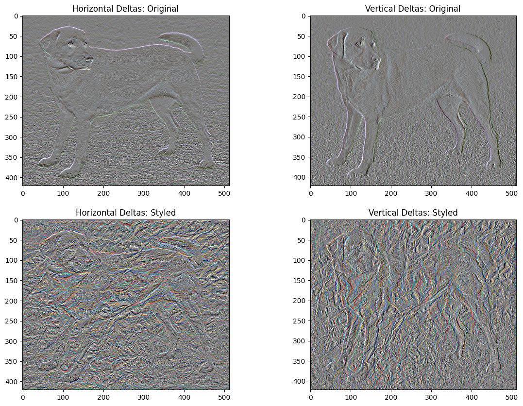
위 이미지들은 고주파 구성 요소가 늘어났다는 것을 보여줍니다.
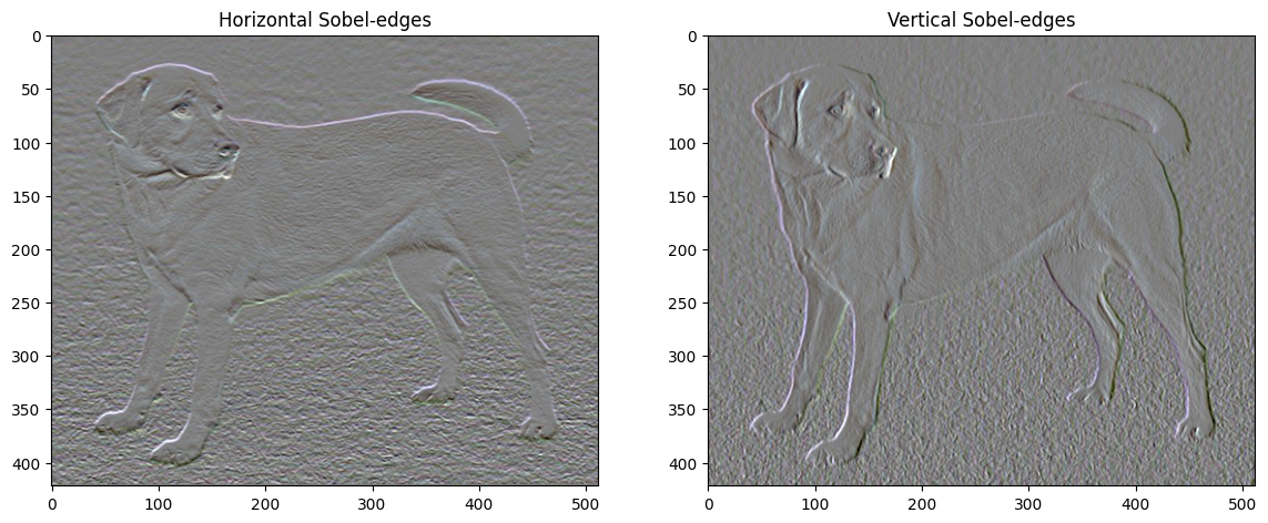
한 가지 흥미로운 사실은 고주파 구성 요소가 경계선 탐지기의 일종이라는 점입니다. 이를테면 소벨 경계선 탐지기(Sobel edge detector)를 사용하면 유사한 출력을 얻을 수 있습니다:
plt.figure(figsize=(14, 10))

sobel = tf.image.sobel_edges(content_image)
plt.subplot(1, 2, 1)
imshow(clip_0_1(sobel[..., 0]/4+0.5), "Horizontal Sobel-edges")
plt.subplot(1, 2, 2)
imshow(clip_0_1(sobel[..., 1]/4+0.5), "Vertical Sobel-edges")
정규화 오차는 각 값의 절대값의 합으로 표현됩니다:
def total_variation_loss(image):
  x_deltas, y_deltas = high_pass_x_y(image)
  return tf.reduce_sum(tf.abs(x_deltas)) + tf.reduce_sum(tf.abs(y_deltas))
total_variation_loss(image).numpy()
149222.6
식이 잘 계산된다는 것을 확인할 수 있습니다. 하지만 다행히도 텐서플로에는 이미 표준 함수가 내장되어 있기 직접 오차식을 구현할 필요는 없습니다:
tf.image.total_variation(image).numpy()
array([149222.6], dtype=float32)
다시 최적화하기
total_variation_loss를 위한 가중치를 정의합니다:
total_variation_weight=30
이제 이 가중치를 train_step 함수에서 사용합니다:
@tf.function()
def train_step(image):
  with tf.GradientTape() as tape:
    outputs = extractor(image)
    loss = style_content_loss(outputs)
    loss += total_variation_weight*tf.image.total_variation(image)

  grad = tape.gradient(loss, image)
  opt.apply_gradients([(grad, image)])
  image.assign(clip_0_1(image))
이미지 변수와 옵티마이저를 다시 초기화합니다.
opt = tf.keras.optimizers.Adam(learning_rate=0.02, beta_1=0.99, epsilon=1e-1)
image = tf.Variable(content_image)
최적화를 수행합니다:
import time
start = time.time()
epochs = 10
steps_per_epoch = 100
step = 0
for n in range(epochs):
for m in range(steps_per_epoch):
step += 1
train_step(image)
print(".", end='', flush=True)
display.clear_output(wait=True)
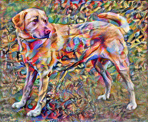
display.display(tensor_to_image(image))
print("Train step: {}".format(step))
end = time.time()
print("Total time: {:.1f}".format(end-start))
Train step: 1000
Total time: 36.8
마지막으로, 결과물을 저장합니다:
file_name = 'stylized-image.png'
tensor_to_image(image).save(file_name)

try:
  from google.colab import files
except ImportError:
   pass
else:
  files.download(file_name)
자세히 알아보기
이 튜토리얼은 원래 스타일 전송 알고리즘을 보여줍니다. 스타일 전송의 간단한 적용에 대해서는 이 튜토리얼을 확인하여 TensorFlow Hub에서 임의의 이미지 스타일 전송 모델을 사용하는 방법에 대해 자세히 알아보세요.