
| |
 GitHub에서 소스 보기 GitHub에서 소스 보기 |
이 튜토리얼은 수정된 U-Net을 사용하여 이미지 분할 작업에 중점을 둡니다.
이미지 분할이란?
이미지 분류 작업에서 네트워크는 각 입력 이미지에 레이블(또는 클래스)을 할당합니다. 그러나 해당 객체의 모양, 어떤 픽셀이 어떤 객체에 속하는지 등을 알고 싶다고 가정해 보겠습니다. 이 경우 이미지의 각 픽셀에 클래스를 할당해야 할 것입니다. 이 작업을 세분화라고 합니다. 세분화 모델은 이미지에 대한 훨씬 더 자세한 정보를 반환합니다. 이미지 분할은 의료 영상, 자율 주행 자동차, 위성 영상 등 여러 분야에 응용됩니다.
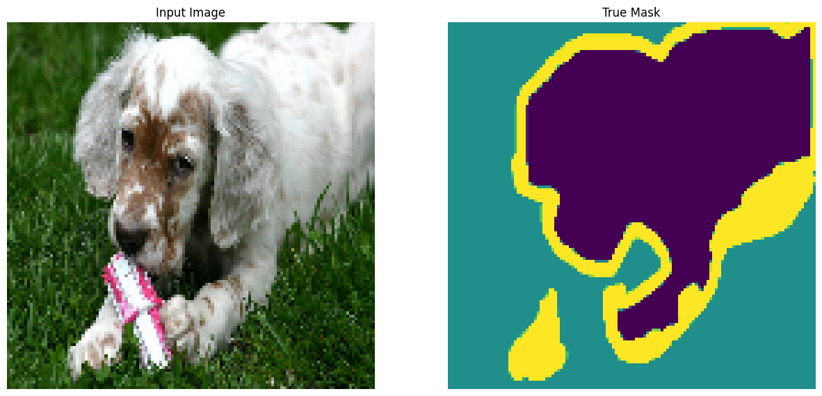
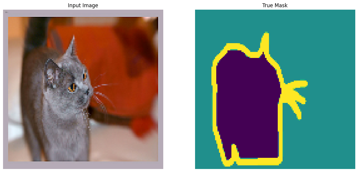
이 튜토리얼은 Oxford-IIIT Pet Dataset(Parkhi 등, 2012)을 사용합니다. 이 데이터세트는 37개의 애완동물 품종의 이미지로 구성되어 있으며 품종당 200개의 이미지가 있습니다(훈련 및 테스트 분할에 각각 ~100개). 각 이미지에는 해당 레이블과 픽셀 단위 마스크가 포함됩니다. 마스크는 각 픽셀에 대한 클래스 레이블입니다. 각 픽셀에는 세 가지 범주 중 하나가 지정됩니다.
- 클래스 1: 애완 동물에 속하는 픽셀
- 클래스 2: 애완동물과 접하는 픽셀
- 클래스 3: 위에 속하지 않음/주변 픽셀
pip install git+https://github.com/tensorflow/examples.gitimport tensorflow as tf
import tensorflow_datasets as tfds
2022-12-15 01:31:46.762319: W tensorflow/compiler/xla/stream_executor/platform/default/dso_loader.cc:64] Could not load dynamic library 'libnvinfer.so.7'; dlerror: libnvinfer.so.7: cannot open shared object file: No such file or directory
2022-12-15 01:31:46.762438: W tensorflow/compiler/xla/stream_executor/platform/default/dso_loader.cc:64] Could not load dynamic library 'libnvinfer_plugin.so.7'; dlerror: libnvinfer_plugin.so.7: cannot open shared object file: No such file or directory
2022-12-15 01:31:46.762448: W tensorflow/compiler/tf2tensorrt/utils/py_utils.cc:38] TF-TRT Warning: Cannot dlopen some TensorRT libraries. If you would like to use Nvidia GPU with TensorRT, please make sure the missing libraries mentioned above are installed properly.
from tensorflow_examples.models.pix2pix import pix2pix

from IPython.display import clear_output
import matplotlib.pyplot as plt
Oxford-IIIT Pets 데이터 세트를 다운로드 하기
데이터세트는 TensorFlow Datasets에서 사용할 수 있습니다. 세분화 마스크는 버전 3+에 포함되어 있습니다.
dataset, info = tfds.load('oxford_iiit_pet:3.*.*', with_info=True)
또한 이미지 색상 값은 [0,1] 범위로 정규화됩니다. 마지막으로 위에서 언급한 것처럼 분할 마스크의 픽셀에는 {1, 2, 3}이라는 레이블이 지정됩니다. 편의를 위해 세분화 마스크에서 1을 빼면 {0, 1, 2}와 같은 레이블이 생성됩니다.
def normalize(input_image, input_mask):
  input_image = tf.cast(input_image, tf.float32) / 255.0
  input_mask -= 1
  return input_image, input_mask
def load_image(datapoint):
  input_image = tf.image.resize(datapoint['image'], (128, 128))
  input_mask = tf.image.resize(datapoint['segmentation_mask'], (128, 128))

  input_image, input_mask = normalize(input_image, input_mask)

  return input_image, input_mask
데이터세트에는 이미 필요한 훈련 및 테스트 분할이 포함되어 있으므로 동일한 분할을 계속 사용하세요.
TRAIN_LENGTH = info.splits['train'].num_examples
BATCH_SIZE = 64
BUFFER_SIZE = 1000
STEPS_PER_EPOCH = TRAIN_LENGTH // BATCH_SIZE
train_images = dataset['train'].map(load_image, num_parallel_calls=tf.data.AUTOTUNE)
test_images = dataset['test'].map(load_image, num_parallel_calls=tf.data.AUTOTUNE)
다음 클래스는 이미지를 무작위로 뒤집어 간단한 증강을 수행합니다. 자세히 알아보려면 이미지 증강 튜토리얼로 이동하세요.
class Augment(tf.keras.layers.Layer):
  def __init__(self, seed=42):
    super().__init__()
    # both use the same seed, so they'll make the same random changes.
    self.augment_inputs = tf.keras.layers.RandomFlip(mode="horizontal", seed=seed)
    self.augment_labels = tf.keras.layers.RandomFlip(mode="horizontal", seed=seed)

  def call(self, inputs, labels):
    inputs = self.augment_inputs(inputs)
    labels = self.augment_labels(labels)
    return inputs, labels
입력을 일괄 처리한 후 증강을 적용하여 입력 파이프라인을 빌드합니다.
train_batches = (
    train_images
    .cache()
    .shuffle(BUFFER_SIZE)
    .batch(BATCH_SIZE)
    .repeat()
    .map(Augment())
    .prefetch(buffer_size=tf.data.AUTOTUNE))

test_batches = test_images.batch(BATCH_SIZE)
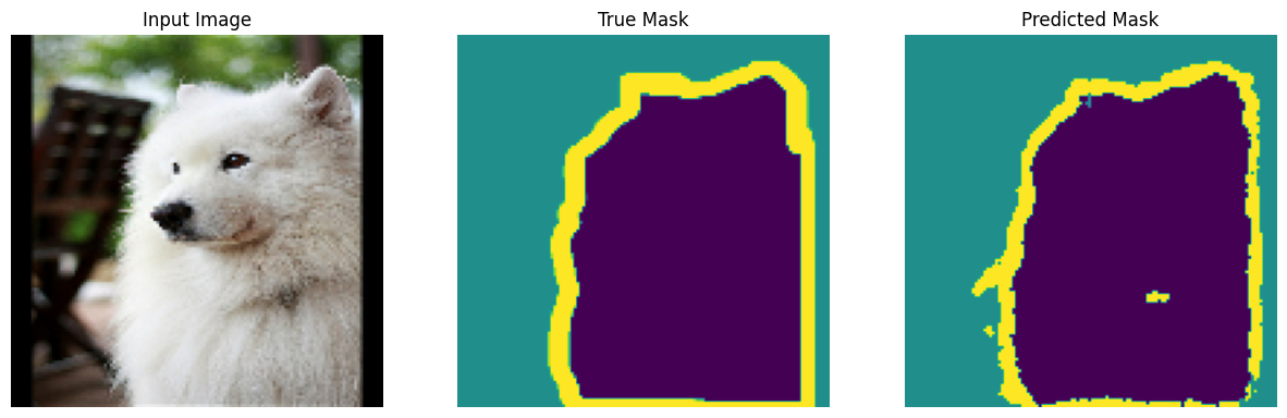
데이터세트에서 이미지 예제와 해당 마스크를 시각화합니다.
def display(display_list):
  plt.figure(figsize=(15, 15))

  title = ['Input Image', 'True Mask', 'Predicted Mask']

  for i in range(len(display_list)):
    plt.subplot(1, len(display_list), i+1)
    plt.title(title[i])
    plt.imshow(tf.keras.utils.array_to_img(display_list[i]))
    plt.axis('off')
  plt.show()
for images, masks in train_batches.take(2):
  sample_image, sample_mask = images[0], masks[0]
  display([sample_image, sample_mask])
Corrupt JPEG data: 240 extraneous bytes before marker 0xd9
Corrupt JPEG data: premature end of data segment
2022-12-15 01:31:56.134500: W tensorflow/core/kernels/data/cache_dataset_ops.cc:856] The calling iterator did not fully read the dataset being cached. In order to avoid unexpected truncation of the dataset, the partially cached contents of the dataset will be discarded. This can happen if you have an input pipeline similar to `dataset.cache().take(k).repeat()`. You should use `dataset.take(k).cache().repeat()` instead.
모델 정의하기
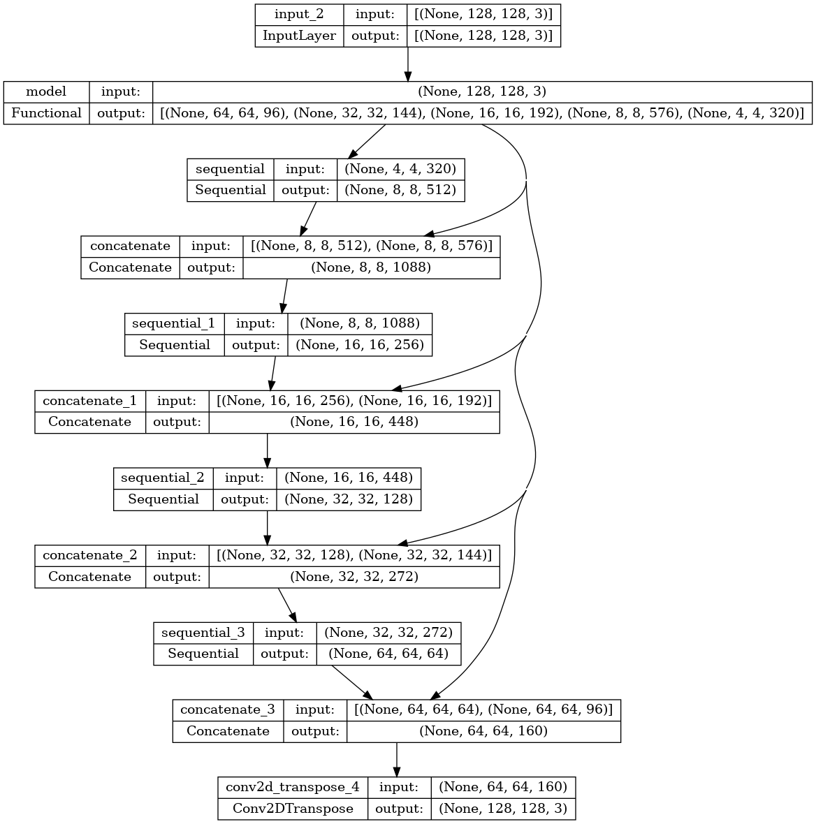
여기에 사용된 모델은 수정된 U-Net입니다. U-Net은 인코더(다운샘플러)와 디코더(업샘플러)로 구성됩니다. 강력한 기능을 학습하고 학습 가능한 매개변수의 수를 줄이기 위해 사전 학습된 모델인 MobileNetV2를 인코더로 사용합니다. 디코더의 경우 TensorFlow 예제 리포지토리의 pix2pix 예제에서 이미 구현된 업샘플 블록을 사용합니다. 노트북에서 pix2pix: 조건부 GAN을 사용한 이미지 대 이미지 변환 튜토리얼을 확인하세요.
언급했듯이 인코더는 사전 학습된 MobileNetV2 모델입니다. tf.keras.applications의 모델을 사용합니다. 인코더는 모델의 중간 레이어에서 얻어지는 특정 출력으로 구성됩니다. 인코더는 학습 과정에서 훈련되지 않습니다.
base_model = tf.keras.applications.MobileNetV2(input_shape=[128, 128, 3], include_top=False)

# Use the activations of these layers
layer_names = [
    'block_1_expand_relu',   # 64x64
    'block_3_expand_relu',   # 32x32
    'block_6_expand_relu',   # 16x16
    'block_13_expand_relu',  # 8x8
    'block_16_project',      # 4x4
]
base_model_outputs = [base_model.get_layer(name).output for name in layer_names]

# Create the feature extraction model
down_stack = tf.keras.Model(inputs=base_model.input, outputs=base_model_outputs)

down_stack.trainable = False
Downloading data from https://storage.googleapis.com/tensorflow/keras-applications/mobilenet_v2/mobilenet_v2_weights_tf_dim_ordering_tf_kernels_1.0_128_no_top.h5
9406464/9406464 [==============================] - 0s 0us/step
디코더/업샘플러는 TensorFlow 예제에서 구현된 일련의 업샘플 블록입니다.
up_stack = [
    pix2pix.upsample(512, 3),  # 4x4 -> 8x8
    pix2pix.upsample(256, 3),  # 8x8 -> 16x16
    pix2pix.upsample(128, 3),  # 16x16 -> 32x32
    pix2pix.upsample(64, 3),   # 32x32 -> 64x64
]
def unet_model(output_channels:int):
  inputs = tf.keras.layers.Input(shape=[128, 128, 3])

  # Downsampling through the model
  skips = down_stack(inputs)
  x = skips[-1]
  skips = reversed(skips[:-1])

  # Upsampling and establishing the skip connections
  for up, skip in zip(up_stack, skips):
    x = up(x)
    concat = tf.keras.layers.Concatenate()
    x = concat([x, skip])

  # This is the last layer of the model
  last = tf.keras.layers.Conv2DTranspose(
      filters=output_channels, kernel_size=3, strides=2,
      padding='same')  #64x64 -> 128x128

  x = last(x)

  return tf.keras.Model(inputs=inputs, outputs=x)
마지막 레이어의 필터 수는 output_channels의 수로 설정됩니다. 이것은 클래스당 하나의 출력 채널이 됩니다.
모델 훈련하기
이제 모델을 컴파일하고 훈련하는 일만 남았습니다.
이것은 다중 클래스 분류 문제이므로 from_logits 인수가 True로 설정된 tf.keras.losses.CategoricalCrossentropy 손실 함수를 사용하세요. 레이블은 모든 클래스의 각 픽셀에 대한 점수 벡터가 아니라 정수 스칼라이기 때문입니다.
추론을 실행할 때 픽셀에 할당된 레이블은 값이 가장 높은 채널입니다. 이것이 create_mask 함수가 하는 일입니다.
OUTPUT_CLASSES = 3

model = unet_model(output_channels=OUTPUT_CLASSES)
model.compile(optimizer='adam',
              loss=tf.keras.losses.SparseCategoricalCrossentropy(from_logits=True),
              metrics=['accuracy'])
결과적인 모델 아키텍처를 플로팅합니다.
tf.keras.utils.plot_model(model, show_shapes=True)
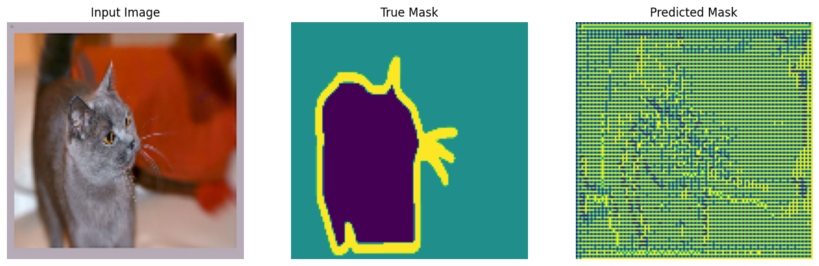
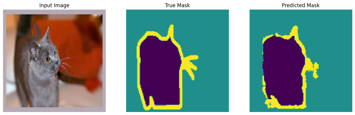
훈련 전에 모델이 예측하는 것을 확인하기 위해 모델을 시험해 보세요.
def create_mask(pred_mask):
  pred_mask = tf.math.argmax(pred_mask, axis=-1)
  pred_mask = pred_mask[..., tf.newaxis]
  return pred_mask[0]
def show_predictions(dataset=None, num=1):
  if dataset:
    for image, mask in dataset.take(num):
      pred_mask = model.predict(image)
      display([image[0], mask[0], create_mask(pred_mask)])
  else:
    display([sample_image, sample_mask,
             create_mask(model.predict(sample_image[tf.newaxis, ...]))])
show_predictions()
1/1 [==============================] - 2s 2s/step
아래에 정의된 콜백은 모델이 훈련되는 동안 어떻게 개선되는지 관찰하는 데 사용됩니다.
class DisplayCallback(tf.keras.callbacks.Callback):
  def on_epoch_end(self, epoch, logs=None):
    clear_output(wait=True)
    show_predictions()
    print ('\nSample Prediction after epoch {}\n'.format(epoch+1))
EPOCHS = 20
VAL_SUBSPLITS = 5
VALIDATION_STEPS = info.splits['test'].num_examples//BATCH_SIZE//VAL_SUBSPLITS

model_history = model.fit(train_batches, epochs=EPOCHS,
                          steps_per_epoch=STEPS_PER_EPOCH,
                          validation_steps=VALIDATION_STEPS,
                          validation_data=test_batches,
                          callbacks=[DisplayCallback()])
1/1 [==============================] - 0s 30ms/step
Sample Prediction after epoch 20

57/57 [==============================] - 5s 94ms/step - loss: 0.1321 - accuracy: 0.9396 - val_loss: 0.3194 - val_accuracy: 0.8891
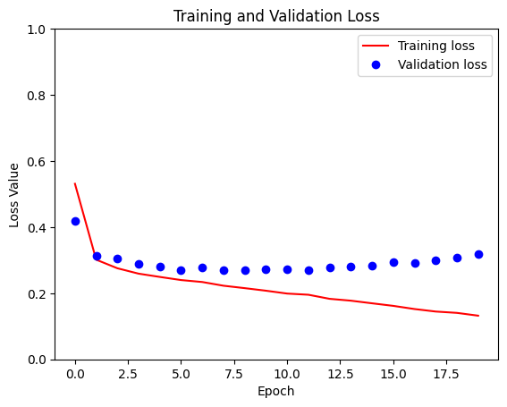
loss = model_history.history['loss']
val_loss = model_history.history['val_loss']

plt.figure()
plt.plot(model_history.epoch, loss, 'r', label='Training loss')
plt.plot(model_history.epoch, val_loss, 'bo', label='Validation loss')
plt.title('Training and Validation Loss')
plt.xlabel('Epoch')
plt.ylabel('Loss Value')
plt.ylim([0, 1])
plt.legend()
plt.show()
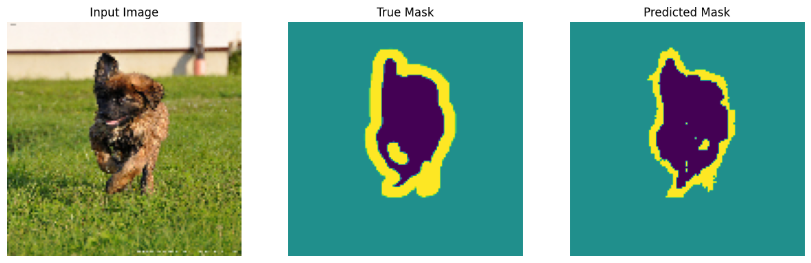
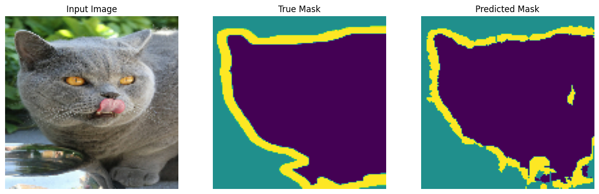
예측하기
이제 몇 가지 예측을 하겠습니다. 시간을 절약하기 위해 epoch 수를 작게 유지했지만 더 정확한 결과를 얻으려면 이 값을 더 높게 설정할 수 있습니다.
show_predictions(test_batches, 3)
2/2 [==============================] - 0s 21ms/step
2/2 [==============================] - 0s 21ms/step
2/2 [==============================] - 0s 21ms/step
옵션: 불균형 클래스 및 클래스 가중치
시맨틱 분할 데이터세트는 불균형이 심할 수 있습니다. 즉, 특정 클래스 픽셀이 다른 클래스의 픽셀보다 이미지 내부에 더 많이 존재할 수 있습니다. 분할 문제는 픽셀별 분류 문제로 취급될 수 있으므로, 이를 설명하기 위해 손실 함수에 가중치를 주어 불균형 문제를 처리할 수 있습니다. 이것이 이 문제를 처리하는 간단하고 무리 없는 방법입니다. 자세한 내용은 불균형 데이터에 대한 분류 튜토리얼을 참조하세요.
모호성을 피하기 위해 Model.fit은 3차원 이상의 입력에 대해 class_weight 인수를 지원하지 않습니다.
try:
  model_history = model.fit(train_batches, epochs=EPOCHS,
                            steps_per_epoch=STEPS_PER_EPOCH,
                            class_weight = {0:2.0, 1:2.0, 2:1.0})
  assert False
except Exception as e:
  print(f"Expected {type(e).__name__}: {e}")
Expected ValueError: `class_weight` not supported for 3+ dimensional targets.
따라서 이 경우 가중치를 직접 구현해야 합니다. 샘플 가중치를 사용하여 이 작업을 수행합니다. (data, label) 쌍 외에 Model.fit는 (data, label, sample_weight) 트리플도 허용합니다.
Keras Model.fit은 sample_weight를 손실 및 메트릭으로 전파하며 sample_weight 인수도 허용합니다. 샘플 가중치는 감소 단계 이전의 샘플 값으로 곱해집니다. 예를 들면 다음과 같습니다.
label = [0,0]
prediction = [[-3., 0], [-3, 0]]
sample_weight = [1, 10]

loss = tf.keras.losses.SparseCategoricalCrossentropy(from_logits=True,
                                               reduction=tf.keras.losses.Reduction.NONE)
loss(label, prediction, sample_weight).numpy()
array([ 3.0485873, 30.485874 ], dtype=float32)
따라서 이 튜토리얼을 위한 샘플 가중치를 만들려면 (data, label) 쌍을 받아서 (data, label, sample_weight) 트리플을 반환하는 함수가 필요합니다. 여기서 sample_weight는 각 픽셀에 대한 클래스 가중치를 포함하는 1채널 이미지입니다.
가장 간단한 구현은 레이블을 class_weight 목록에 대한 인덱스로 사용하는 것입니다.
def add_sample_weights(image, label):
  # The weights for each class, with the constraint that:
  #     sum(class_weights) == 1.0
  class_weights = tf.constant([2.0, 2.0, 1.0])
  class_weights = class_weights/tf.reduce_sum(class_weights)

  # Create an image of `sample_weights` by using the label at each pixel as an
  # index into the `class weights` .
  sample_weights = tf.gather(class_weights, indices=tf.cast(label, tf.int32))

  return image, label, sample_weights
결과 데이터세트 요소에는 각각 3개의 이미지가 포함됩니다.
train_batches.map(add_sample_weights).element_spec
(TensorSpec(shape=(None, 128, 128, 3), dtype=tf.float32, name=None),
 TensorSpec(shape=(None, 128, 128, 1), dtype=tf.float32, name=None),
 TensorSpec(shape=(None, 128, 128, 1), dtype=tf.float32, name=None))
이제 가중치 적용된 이 데이터세트에서 모델을 훈련할 수 있습니다.
weighted_model = unet_model(OUTPUT_CLASSES)
weighted_model.compile(
    optimizer='adam',
    loss=tf.keras.losses.SparseCategoricalCrossentropy(from_logits=True),
    metrics=['accuracy'])
weighted_model.fit(
    train_batches.map(add_sample_weights),
    epochs=1,
    steps_per_epoch=10)
10/10 [==============================] - 5s 72ms/step - loss: 0.2798 - accuracy: 0.6679
<keras.callbacks.History at 0x7f619e1b9190>
다음 단계
이제 이미지 분할이 무엇이며 어떻게 작동하는지 이해했으므로 다른 중간 레이어 출력 또는 다른 사전 훈련된 모델을 사용하여 이 튜토리얼을 시험해 볼 수 있습니다. Kaggle에서 호스팅되는 Carvana 이미지 마스킹 챌린지를 통해 자신을 테스트해볼 수도 있습니다.
자체 데이터에 대해 재학습할 수 있는 다른 모델에 대한 Tensorflow Object Detection API를 보고 싶을 수도 있을 것입니다. TensorFlow Hub에서 사전 훈련된 모델을 사용할 수 있습니다.