
 GitHub에서 소스 보기 GitHub에서 소스 보기 |
이 텍스트 분류 튜토리얼은 감정 분석을 위해 IMDB 대형 영화 리뷰 데이터세트로 순환 신경망을 훈련합니다.
설정
pip install -q tfds-nightlyimport tensorflow_datasets as tfds
import tensorflow as tf
2022-12-14 21:32:10.783130: W tensorflow/compiler/xla/stream_executor/platform/default/dso_loader.cc:64] Could not load dynamic library 'libnvinfer.so.7'; dlerror: libnvinfer.so.7: cannot open shared object file: No such file or directory
2022-12-14 21:32:10.783247: W tensorflow/compiler/xla/stream_executor/platform/default/dso_loader.cc:64] Could not load dynamic library 'libnvinfer_plugin.so.7'; dlerror: libnvinfer_plugin.so.7: cannot open shared object file: No such file or directory
2022-12-14 21:32:10.783258: W tensorflow/compiler/tf2tensorrt/utils/py_utils.cc:38] TF-TRT Warning: Cannot dlopen some TensorRT libraries. If you would like to use Nvidia GPU with TensorRT, please make sure the missing libraries mentioned above are installed properly.
matplotlib을 가져오고 그래프를 플롯하는 helper 함수를 만듭니다.
import matplotlib.pyplot as plt

def plot_graphs(history, metric):
  plt.plot(history.history[metric])
  plt.plot(history.history['val_'+metric], '')
  plt.xlabel("Epochs")
  plt.ylabel(metric)
  plt.legend([metric, 'val_'+metric])
  plt.show()
입력 파이프라인 설정하기
IMDB 대형 영화 리뷰 데이터세트는 binary classification 데이터세트입니다. 모든 리뷰에는 positive 또는 negative 감정이 있습니다.
TFDS를 사용하여 데이터세트를 다운로드합니다.
dataset, info = tfds.load('imdb_reviews/subwords8k', with_info=True,
                          as_supervised=True)
train_dataset, test_dataset = dataset['train'], dataset['test']
WARNING:absl:TFDS datasets with text encoding are deprecated and will be removed in a future version. Instead, you should use the plain text version and tokenize the text using `tensorflow_text` (See: https://www.tensorflow.org/tutorials/tensorflow_text/intro#tfdata_example)
데이터세트 info에는 인코더( tfds.features.text.SubwordTextEncoder)가 포함됩니다.
encoder = info.features['text'].encoder
print('Vocabulary size: {}'.format(encoder.vocab_size))
Vocabulary size: 8185
이 텍스트 인코더는 문자열을 가역적으로 인코딩하여 필요한 경우 바이트 인코딩으로 돌아갑니다.
sample_string = 'Hello TensorFlow.'

encoded_string = encoder.encode(sample_string)
print('Encoded string is {}'.format(encoded_string))

original_string = encoder.decode(encoded_string)
print('The original string: "{}"'.format(original_string))
Encoded string is [4025, 222, 6307, 2327, 4043, 2120, 7975]
The original string: "Hello TensorFlow."
assert original_string == sample_string
for index in encoded_string:
  print('{} ----> {}'.format(index, encoder.decode([index])))
4025 ----> Hell
222 ----> o
6307 ----> Ten
2327 ----> sor
4043 ----> Fl
2120 ----> ow
7975 ----> .
훈련을 위한 데이터 준비하기
다음으로 이러한 인코딩된 문자열을 일괄적으로 생성합니다. padded_batch 메서드를 사용하여 배치에서 가장 긴 문자열의 길이로 시퀀스를 0으로 채웁니다.
BUFFER_SIZE = 10000
BATCH_SIZE = 64
train_dataset = train_dataset.shuffle(BUFFER_SIZE)
train_dataset = train_dataset.padded_batch(BATCH_SIZE)

test_dataset = test_dataset.padded_batch(BATCH_SIZE)
모델 만들기
tf.keras.Sequential 모델을 빌드하고 embedding 레이어로 시작합니다. embedding 레이어는 단어당 하나의 벡터를 저장합니다. 호출되면 단어 인덱스 시퀀스를 벡터 시퀀스로 변환합니다. 이들 벡터는 훈련 가능합니다. (충분한 데이터에 대해) 훈련 후, 유사한 의미를 가진 단어는 종종 비슷한 벡터를 갖습니다.
이 인덱스 조회는 원-핫 인코딩된 벡터를 tf.keras.layers.Dense 레이어를 통해 전달하는 동등한 연산보다 훨씬 효율적입니다.
RNN(Recurrent Neural Network)은 요소를 반복하여 시퀀스 입력을 처리합니다. RNN은 출력을 하나의 타임스텝에서 입력으로 전달한 다음, 다음 단계로 전달합니다.
tf.keras.layers.Bidirectional 래퍼도 RNN 레이어와 함께 사용할 수 있습니다. 이는 RNN 레이어를 통해 입력을 앞뒤로 전파한 다음 출력을 연결합니다. 이는 RNN이 장거리 종속성을 학습하는 데 도움이 됩니다.
model = tf.keras.Sequential([
    tf.keras.layers.Embedding(encoder.vocab_size, 64),
    tf.keras.layers.Bidirectional(tf.keras.layers.LSTM(64)),
    tf.keras.layers.Dense(64, activation='relu'),
    tf.keras.layers.Dense(1)
])
모델의 모든 레이어에는 단일 입력만 있고 단일 출력이 생성되므로 여기서는 Keras 순차형 모델을 선택합니다. 상태 저장 RNN 레이어를 사용하려는 경우, Keras 함수 API 또는 모델 하위 클래스화를 사용하여 모델을 빌드하여 RNN 레이어 상태를 검색하고 재사용할 수 있습니다. 자세한 내용은 Keras RNN 가이드를 확인하세요.
Keras 모델을 컴파일하여 훈련 프로세스를 구성합니다.
model.compile(loss=tf.keras.losses.BinaryCrossentropy(from_logits=True),
              optimizer=tf.keras.optimizers.Adam(1e-4),
              metrics=['accuracy'])
모델 훈련하기
history = model.fit(train_dataset, epochs=10,
                    validation_data=test_dataset,
                    validation_steps=30)
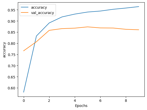
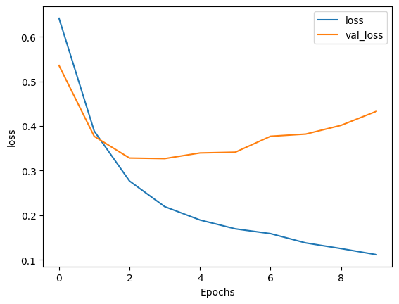
Epoch 1/10
391/391 [==============================] - 91s 218ms/step - loss: 0.6416 - accuracy: 0.5807 - val_loss: 0.5358 - val_accuracy: 0.7661
Epoch 2/10
391/391 [==============================] - 69s 175ms/step - loss: 0.3886 - accuracy: 0.8325 - val_loss: 0.3769 - val_accuracy: 0.8068
Epoch 3/10
391/391 [==============================] - 59s 150ms/step - loss: 0.2767 - accuracy: 0.8910 - val_loss: 0.3281 - val_accuracy: 0.8578
Epoch 4/10
391/391 [==============================] - 55s 140ms/step - loss: 0.2192 - accuracy: 0.9180 - val_loss: 0.3269 - val_accuracy: 0.8656
Epoch 5/10
391/391 [==============================] - 53s 134ms/step - loss: 0.1893 - accuracy: 0.9307 - val_loss: 0.3396 - val_accuracy: 0.8677
Epoch 6/10
391/391 [==============================] - 47s 119ms/step - loss: 0.1695 - accuracy: 0.9399 - val_loss: 0.3413 - val_accuracy: 0.8734
Epoch 7/10
391/391 [==============================] - 46s 116ms/step - loss: 0.1587 - accuracy: 0.9444 - val_loss: 0.3770 - val_accuracy: 0.8687
Epoch 8/10
391/391 [==============================] - 46s 117ms/step - loss: 0.1378 - accuracy: 0.9523 - val_loss: 0.3819 - val_accuracy: 0.8682
Epoch 9/10
391/391 [==============================] - 43s 109ms/step - loss: 0.1252 - accuracy: 0.9579 - val_loss: 0.4016 - val_accuracy: 0.8625
Epoch 10/10
391/391 [==============================] - 44s 111ms/step - loss: 0.1115 - accuracy: 0.9643 - val_loss: 0.4329 - val_accuracy: 0.8604
test_loss, test_acc = model.evaluate(test_dataset)

print('Test Loss: {}'.format(test_loss))
print('Test Accuracy: {}'.format(test_acc))
391/391 [==============================] - 16s 40ms/step - loss: 0.4507 - accuracy: 0.8462
Test Loss: 0.4506881535053253
Test Accuracy: 0.8461999893188477
위의 모델은 시퀀스에 적용된 패딩을 마스킹하지 않습니다. 패딩된 시퀀스에 대해 훈련하고 패딩되지 않은 시퀀스를 테스트하면 왜곡될 수 있습니다. 이상적으로는 마스킹을 사용하여 이를 피할 수 있지만, 아래에서 볼 수 있듯이 출력에는 약간의 영향만 미칩니다.
예측값이 >= 0.5인 경우, 양성이고 그렇지 않으면 음성입니다.
def pad_to_size(vec, size):
  zeros = [0] * (size - len(vec))
  vec.extend(zeros)
  return vec
def sample_predict(sample_pred_text, pad):
  encoded_sample_pred_text = encoder.encode(sample_pred_text)

  if pad:
    encoded_sample_pred_text = pad_to_size(encoded_sample_pred_text, 64)
  encoded_sample_pred_text = tf.cast(encoded_sample_pred_text, tf.float32)
  predictions = model.predict(tf.expand_dims(encoded_sample_pred_text, 0))

  return (predictions)
# predict on a sample text without padding.

sample_pred_text = ('The movie was cool. The animation and the graphics '
                    'were out of this world. I would recommend this movie.')
predictions = sample_predict(sample_pred_text, pad=False)
print(predictions)
1/1 [==============================] - 1s 680ms/step
[[0.05132709]]
# predict on a sample text with padding

sample_pred_text = ('The movie was cool. The animation and the graphics '
                    'were out of this world. I would recommend this movie.')
predictions = sample_predict(sample_pred_text, pad=True)
print(predictions)
1/1 [==============================] - 1s 637ms/step
[[-0.16916835]]
plot_graphs(history, 'accuracy')
plot_graphs(history, 'loss')
두 개 이상의 LSTM 레이어 쌓기
Keras 반복 레이어에는 return_sequences 생성자 인수로 제어되는 두 가지 사용 가능한 모드가 있습니다.
- 각 타임스텝(형상
(batch_size, timesteps, output_features)의 3D 텐서)에 대한 전체 연속 출력 시퀀스를 반환합니다. - 각 입력 시퀀스에 대한 마지막 출력만 반환합니다(형상 (batch_size, output_features)의 2D 텐서).
model = tf.keras.Sequential([
    tf.keras.layers.Embedding(encoder.vocab_size, 64),
    tf.keras.layers.Bidirectional(tf.keras.layers.LSTM(64,  return_sequences=True)),
    tf.keras.layers.Bidirectional(tf.keras.layers.LSTM(32)),
    tf.keras.layers.Dense(64, activation='relu'),
    tf.keras.layers.Dropout(0.5),
    tf.keras.layers.Dense(1)
])
model.compile(loss=tf.keras.losses.BinaryCrossentropy(from_logits=True),
              optimizer=tf.keras.optimizers.Adam(1e-4),
              metrics=['accuracy'])
history = model.fit(train_dataset, epochs=10,
                    validation_data=test_dataset,
                    validation_steps=30)
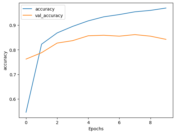
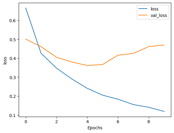
Epoch 1/10
391/391 [==============================] - 113s 271ms/step - loss: 0.6645 - accuracy: 0.5459 - val_loss: 0.5003 - val_accuracy: 0.7620
Epoch 2/10
391/391 [==============================] - 96s 243ms/step - loss: 0.4252 - accuracy: 0.8225 - val_loss: 0.4601 - val_accuracy: 0.7880
Epoch 3/10
391/391 [==============================] - 92s 233ms/step - loss: 0.3475 - accuracy: 0.8683 - val_loss: 0.4050 - val_accuracy: 0.8271
Epoch 4/10
391/391 [==============================] - 89s 226ms/step - loss: 0.2902 - accuracy: 0.8950 - val_loss: 0.3795 - val_accuracy: 0.8370
Epoch 5/10
391/391 [==============================] - 86s 219ms/step - loss: 0.2409 - accuracy: 0.9174 - val_loss: 0.3612 - val_accuracy: 0.8568
Epoch 6/10
391/391 [==============================] - 84s 213ms/step - loss: 0.2048 - accuracy: 0.9338 - val_loss: 0.3664 - val_accuracy: 0.8589
Epoch 7/10
391/391 [==============================] - 83s 210ms/step - loss: 0.1835 - accuracy: 0.9430 - val_loss: 0.4158 - val_accuracy: 0.8552
Epoch 8/10
391/391 [==============================] - 82s 207ms/step - loss: 0.1552 - accuracy: 0.9542 - val_loss: 0.4248 - val_accuracy: 0.8615
Epoch 9/10
391/391 [==============================] - 81s 207ms/step - loss: 0.1409 - accuracy: 0.9600 - val_loss: 0.4611 - val_accuracy: 0.8552
Epoch 10/10
391/391 [==============================] - 81s 205ms/step - loss: 0.1190 - accuracy: 0.9695 - val_loss: 0.4693 - val_accuracy: 0.8422
test_loss, test_acc = model.evaluate(test_dataset)

print('Test Loss: {}'.format(test_loss))
print('Test Accuracy: {}'.format(test_acc))
391/391 [==============================] - 32s 80ms/step - loss: 0.4702 - accuracy: 0.8433
Test Loss: 0.4701811671257019
Test Accuracy: 0.843280017375946
# predict on a sample text without padding.

sample_pred_text = ('The movie was not good. The animation and the graphics '
                    'were terrible. I would not recommend this movie.')
predictions = sample_predict(sample_pred_text, pad=False)
print(predictions)
1/1 [==============================] - 1s 1s/step
[[-2.0136437]]
# predict on a sample text with padding

sample_pred_text = ('The movie was not good. The animation and the graphics '
                    'were terrible. I would not recommend this movie.')
predictions = sample_predict(sample_pred_text, pad=True)
print(predictions)
1/1 [==============================] - 1s 1s/step
[[-2.5655096]]
plot_graphs(history, 'accuracy')
plot_graphs(history, 'loss')
GRU 레이어와 같은 기존의 다른 반복 레이어를 확인합니다.
사용자 정의 RNN 작성에 관심이 있는 경우, Keras RNN 가이드를 참조하세요.