
| | |  ดูแหล่งที่มาบน GitHub ดูแหล่งที่มาบน GitHub | |
ข้อมูล เบื้องต้นเกี่ยวกับการไล่ระดับสีและคู่มือการสร้างความแตกต่างอัตโนมัติ มีทุกอย่างที่จำเป็นในการคำนวณการไล่ระดับสีใน TensorFlow คู่มือนี้เน้นที่คุณลักษณะที่ลึกกว่าและไม่ค่อยพบบ่อยของ tf.GradientTape API
ติดตั้ง
import tensorflow as tf

import matplotlib as mpl
import matplotlib.pyplot as plt

mpl.rcParams['figure.figsize'] = (8, 6)
การควบคุมการบันทึกการไล่ระดับสี
ใน คู่มือการแยกความแตกต่างอัตโนมัติ คุณจะเห็นวิธีควบคุมว่าเทปจะดูตัวแปรและเทนเซอร์ใดขณะสร้างการคำนวณการไล่ระดับสี
เทปยังมีวิธีการจัดการกับการบันทึก
หยุดบันทึก
หากคุณต้องการหยุดบันทึกการไล่ระดับสี คุณสามารถใช้ tf.GradientTape.stop_recording เพื่อระงับการบันทึกชั่วคราว
ซึ่งอาจเป็นประโยชน์ในการลดค่าโสหุ้ย หากคุณไม่ต้องการแยกการทำงานที่ซับซ้อนระหว่างแบบจำลองของคุณ ซึ่งอาจรวมถึงการคำนวณเมตริกหรือผลลัพธ์ขั้นกลาง:
x = tf.Variable(2.0)
y = tf.Variable(3.0)

with tf.GradientTape() as t:
  x_sq = x * x
  with t.stop_recording():
    y_sq = y * y
  z = x_sq + y_sq

grad = t.gradient(z, {'x': x, 'y': y})

print('dz/dx:', grad['x'])  # 2*x => 4
print('dz/dy:', grad['y'])
dz/dx: tf.Tensor(4.0, shape=(), dtype=float32)
dz/dy: None
รีเซ็ต/เริ่มการบันทึกตั้งแต่เริ่มต้น
หากคุณต้องการเริ่มต้นใหม่ทั้งหมด ให้ใช้ tf.GradientTape.reset การออกจากบล็อคเทปแบบเกรเดียนท์และการเริ่มต้นใหม่มักจะง่ายต่อการอ่าน แต่คุณสามารถใช้วิธีการ reset เมื่อออกจากบล็อคเทปนั้นยากหรือเป็นไปไม่ได้
x = tf.Variable(2.0)
y = tf.Variable(3.0)
reset = True

with tf.GradientTape() as t:
  y_sq = y * y
  if reset:
    # Throw out all the tape recorded so far.
    t.reset()
  z = x * x + y_sq

grad = t.gradient(z, {'x': x, 'y': y})

print('dz/dx:', grad['x'])  # 2*x => 4
print('dz/dy:', grad['y'])
dz/dx: tf.Tensor(4.0, shape=(), dtype=float32)
dz/dy: None
หยุดการไหลแบบไล่ระดับด้วยความแม่นยำ
ตรงกันข้ามกับตัวควบคุมเทปทั่วโลกด้านบน ฟังก์ชัน tf.stop_gradient มีความแม่นยำมากกว่ามาก สามารถใช้เพื่อหยุดการไล่ระดับไม่ให้ไหลไปตามเส้นทางใดเส้นทางหนึ่ง โดยไม่ต้องเข้าถึงตัวเทปเอง:
x = tf.Variable(2.0)
y = tf.Variable(3.0)

with tf.GradientTape() as t:
  y_sq = y**2
  z = x**2 + tf.stop_gradient(y_sq)

grad = t.gradient(z, {'x': x, 'y': y})

print('dz/dx:', grad['x'])  # 2*x => 4
print('dz/dy:', grad['y'])
dz/dx: tf.Tensor(4.0, shape=(), dtype=float32)
dz/dy: None
การไล่ระดับสีแบบกำหนดเอง
ในบางกรณี คุณอาจต้องการควบคุมวิธีคำนวณการไล่ระดับสีอย่างแน่ชัด แทนที่จะใช้ค่าเริ่มต้น สถานการณ์เหล่านี้รวมถึง:
- ไม่มีการไล่ระดับสีที่กำหนดไว้สำหรับ op ใหม่ที่คุณกำลังเขียน
- การคำนวณเริ่มต้นเป็นตัวเลขที่ไม่เสถียร
- คุณต้องการแคชการคำนวณที่มีราคาแพงจากการส่งต่อ
- คุณต้องการแก้ไขค่า (เช่น ใช้
tf.clip_by_valueหรือtf.math.round) โดยไม่ต้องแก้ไขการไล่ระดับสี
สำหรับกรณีแรก ในการเขียน op ใหม่ คุณสามารถใช้ tf.RegisterGradient เพื่อตั้งค่าของคุณเองได้ (โปรดดูรายละเอียดในเอกสาร API) (โปรดทราบว่ารีจิสตรีการไล่ระดับสีเป็นแบบโกลบอล ดังนั้นควรเปลี่ยนด้วยความระมัดระวัง)
สำหรับสามกรณีหลัง คุณสามารถใช้ tf.custom_gradient
นี่คือตัวอย่างที่ใช้ tf.clip_by_norm กับการไล่ระดับสีระดับกลาง:
# Establish an identity operation, but clip during the gradient pass.
@tf.custom_gradient
def clip_gradients(y):
  def backward(dy):
    return tf.clip_by_norm(dy, 0.5)
  return y, backward

v = tf.Variable(2.0)
with tf.GradientTape() as t:
  output = clip_gradients(v * v)
print(t.gradient(output, v))  # calls "backward", which clips 4 to 2
tf.Tensor(2.0, shape=(), dtype=float32)
อ้างถึงเอกสาร API ของมัณฑนากร tf.custom_gradient สำหรับรายละเอียดเพิ่มเติม
การไล่ระดับสีแบบกำหนดเองใน SavedModel
สามารถบันทึกการไล่ระดับสีที่กำหนดเองไปที่ SavedModel โดยใช้ตัวเลือก tf.saved_model.SaveOptions(experimental_custom_gradients=True)
หากต้องการบันทึกลงใน SavedModel ฟังก์ชันการไล่ระดับสีจะต้องตรวจสอบย้อนกลับได้ (หากต้องการเรียนรู้เพิ่มเติม โปรดดูคู่มือ ประสิทธิภาพที่ ดีขึ้นด้วย tf.function )
class MyModule(tf.Module):

  @tf.function(input_signature=[tf.TensorSpec(None)])
  def call_custom_grad(self, x):
    return clip_gradients(x)

model = MyModule()
tf.saved_model.save(
    model,
    'saved_model',
    options=tf.saved_model.SaveOptions(experimental_custom_gradients=True))

# The loaded gradients will be the same as the above example.
v = tf.Variable(2.0)
loaded = tf.saved_model.load('saved_model')
with tf.GradientTape() as t:
  output = loaded.call_custom_grad(v * v)
print(t.gradient(output, v))
INFO:tensorflow:Assets written to: saved_model/assets
tf.Tensor(2.0, shape=(), dtype=float32)
หมายเหตุเกี่ยวกับตัวอย่างข้างต้น: หากคุณลองแทนที่โค้ดด้านบนด้วย tf.saved_model.SaveOptions(experimental_custom_gradients=False) การไล่ระดับสีจะยังคงให้ผลลัพธ์แบบเดียวกันเมื่อโหลด เหตุผลก็คือรีจิสทรีการไล่ระดับสียังคงมีการไล่ระดับสีแบบกำหนดเองที่ใช้ในฟังก์ชัน call_custom_op อย่างไรก็ตาม หากคุณเริ่มรันไทม์ใหม่หลังจากบันทึกโดยไม่มีการไล่ระดับสีแบบกำหนดเอง การเรียกใช้โมเดลที่โหลดภายใต้ tf.GradientTape จะแสดงข้อผิดพลาด: LookupError: No gradient defined for operation 'IdentityN' (op type: IdentityN)
หลายเทป
เทปหลายอันโต้ตอบได้อย่างลงตัว
ตัวอย่างเช่น ที่นี่แต่ละเทปดูชุดเมตริกซ์ที่แตกต่างกัน:
x0 = tf.constant(0.0)
x1 = tf.constant(0.0)

with tf.GradientTape() as tape0, tf.GradientTape() as tape1:
  tape0.watch(x0)
  tape1.watch(x1)

  y0 = tf.math.sin(x0)
  y1 = tf.nn.sigmoid(x1)

  y = y0 + y1

  ys = tf.reduce_sum(y)
tape0.gradient(ys, x0).numpy() # cos(x) => 1.0
1.0
tape1.gradient(ys, x1).numpy() # sigmoid(x1)*(1-sigmoid(x1)) => 0.25
0.25
การไล่ระดับสีขั้นสูง
การดำเนินการภายในตัวจัดการบริบท tf.GradientTape จะถูกบันทึกสำหรับการสร้างความแตกต่างโดยอัตโนมัติ หากคำนวณการไล่ระดับสีในบริบทนั้น การคำนวณการไล่ระดับสีก็จะถูกบันทึกเช่นกัน ด้วยเหตุนี้ API เดียวกันจึงทำงานสำหรับการไล่ระดับลำดับที่สูงกว่าเช่นกัน
ตัวอย่างเช่น:
x = tf.Variable(1.0)  # Create a Tensorflow variable initialized to 1.0

with tf.GradientTape() as t2:
  with tf.GradientTape() as t1:
    y = x * x * x

  # Compute the gradient inside the outer `t2` context manager
  # which means the gradient computation is differentiable as well.
  dy_dx = t1.gradient(y, x)
d2y_dx2 = t2.gradient(dy_dx, x)

print('dy_dx:', dy_dx.numpy())  # 3 * x**2 => 3.0
print('d2y_dx2:', d2y_dx2.numpy())  # 6 * x => 6.0
dy_dx: 3.0
d2y_dx2: 6.0
แม้ว่าจะให้อนุพันธ์อันดับสองของฟังก์ชัน สเกลาร์ แต่รูปแบบนี้ไม่ได้สร้างเมทริกซ์แบบเฮสเซียน เนื่องจาก tf.GradientTape.gradient คำนวณเฉพาะการไล่ระดับสีของสเกลาร์ ในการสร้าง เมทริกซ์ Hessian ไปที่ ตัวอย่าง Hessian ใต้ ส่วน Jacobian
"การเรียกแบบซ้อนไปยัง tf.GradientTape.gradient " เป็นรูปแบบที่ดีเมื่อคุณคำนวณสเกลาร์จากการไล่ระดับสี จากนั้นสเกลาร์ที่ได้จะทำหน้าที่เป็นแหล่งสำหรับการคำนวณการไล่ระดับสีที่สอง ดังในตัวอย่างต่อไปนี้
ตัวอย่าง: การทำให้เป็นมาตรฐานการไล่ระดับสีอินพุต
หลายรุ่นมีความอ่อนไหวต่อ "ตัวอย่างที่เป็นปฏิปักษ์" คอลเล็กชันเทคนิคนี้จะปรับเปลี่ยนข้อมูลเข้าของโมเดลเพื่อทำให้เอาต์พุตของโมเดลสับสน การใช้งานที่ง่ายที่สุด—เช่น ตัวอย่าง Adversarial โดยใช้การโจมตี Fast Gradient Signed Method—ใช้ขั้นตอนเดียวตามไล่ระดับของเอาต์พุตที่สัมพันธ์กับอินพุต "การไล่ระดับสีอินพุต"
เทคนิคหนึ่งในการเพิ่มความคงทนให้กับตัวอย่างที่เป็นปฏิปักษ์คือการปรับเกร เดียนต์ของอินพุต ให้เป็นมาตรฐาน (Finlay & Oberman, 2019) ซึ่งพยายามลดขนาดของเกรเดียนต์อินพุตให้น้อยที่สุด หากการไล่ระดับสีอินพุตมีขนาดเล็ก การเปลี่ยนแปลงในเอาต์พุตก็ควรมีขนาดเล็กเช่นกัน
ด้านล่างนี้คือการดำเนินการอย่างไร้เดียงสาของการทำให้เป็นมาตรฐานการไล่ระดับสีอินพุต การดำเนินการคือ:
- คำนวณความลาดชันของเอาต์พุตที่สัมพันธ์กับอินพุตโดยใช้เทปด้านใน
- คำนวณขนาดของการไล่ระดับอินพุตนั้น
- คำนวณความชันของขนาดนั้นเทียบกับแบบจำลอง
x = tf.random.normal([7, 5])

layer = tf.keras.layers.Dense(10, activation=tf.nn.relu)
with tf.GradientTape() as t2:
  # The inner tape only takes the gradient with respect to the input,
  # not the variables.
  with tf.GradientTape(watch_accessed_variables=False) as t1:
    t1.watch(x)
    y = layer(x)
    out = tf.reduce_sum(layer(x)**2)
  # 1. Calculate the input gradient.
  g1 = t1.gradient(out, x)
  # 2. Calculate the magnitude of the input gradient.
  g1_mag = tf.norm(g1)

# 3. Calculate the gradient of the magnitude with respect to the model.
dg1_mag = t2.gradient(g1_mag, layer.trainable_variables)
[var.shape for var in dg1_mag]
[TensorShape([5, 10]), TensorShape([10])]
จาโคเบียน
ตัวอย่างก่อนหน้านี้ทั้งหมดใช้การไล่ระดับของเป้าหมายสเกลาร์เทียบกับเทนเซอร์ต้นทางบางตัว
เมทริกซ์จาโคเบียน แสดงถึงการไล่ระดับสีของฟังก์ชันค่าเวกเตอร์ แต่ละแถวมีการไล่ระดับสีของหนึ่งในองค์ประกอบของเวกเตอร์
วิธี tf.GradientTape.jacobian ช่วยให้คุณคำนวณเมทริกซ์จาโคเบียนได้อย่างมีประสิทธิภาพ
โปรดทราบว่า:
- Like
gradient: อาร์กิวเมนต์sourcesสามารถเป็นเทนเซอร์หรือคอนเทนเนอร์ของเทนเซอร์ - ไม่เหมือนกับ
gradient: เทนเซอร์targetต้องเป็นเมตริกซ์เดียว
แหล่งสเกลาร์
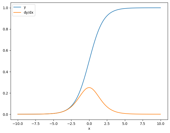
ตัวอย่างแรก นี่คือจาโคเบียนของเป้าหมายเวกเตอร์ที่เกี่ยวกับแหล่งสเกลาร์
x = tf.linspace(-10.0, 10.0, 200+1)
delta = tf.Variable(0.0)

with tf.GradientTape() as tape:
  y = tf.nn.sigmoid(x+delta)

dy_dx = tape.jacobian(y, delta)
เมื่อคุณใช้จาโคเบียนเทียบกับสเกลาร์ ผลลัพธ์จะมีรูปทรงของ เป้าหมาย และให้การไล่ระดับสีของแต่ละองค์ประกอบตามแหล่งที่มา:
print(y.shape)
print(dy_dx.shape)
(201,)
(201,)
plt.plot(x.numpy(), y, label='y')
plt.plot(x.numpy(), dy_dx, label='dy/dx')
plt.legend()
_ = plt.xlabel('x')
แหล่งเทนเซอร์
ไม่ว่าอินพุตจะเป็นสเกลาร์หรือเทนเซอร์ tf.GradientTape.jacobian คำนวณความลาดชันของแต่ละองค์ประกอบของแหล่งที่มาอย่างมีประสิทธิภาพตามแต่ละองค์ประกอบของเป้าหมาย
ตัวอย่างเช่น ผลลัพธ์ของเลเยอร์นี้มีรูปร่างเป็น (10, 7) :
x = tf.random.normal([7, 5])
layer = tf.keras.layers.Dense(10, activation=tf.nn.relu)

with tf.GradientTape(persistent=True) as tape:
  y = layer(x)

y.shape
TensorShape([7, 10])
และรูปร่างของเคอร์เนลของเลเยอร์คือ (5, 10) :
layer.kernel.shape
TensorShape([5, 10])
รูปร่างของจาโคเบียนของเอาต์พุตที่สัมพันธ์กับเคอร์เนลคือรูปร่างทั้งสองที่ต่อกัน:
j = tape.jacobian(y, layer.kernel)
j.shape
TensorShape([7, 10, 5, 10])ตัวยึดตำแหน่ง33
หากคุณรวมขนาดของเป้าหมาย คุณจะเหลือการไล่ระดับสีของผลรวมที่จะคำนวณโดย tf.GradientTape.gradient :
g = tape.gradient(y, layer.kernel)
print('g.shape:', g.shape)

j_sum = tf.reduce_sum(j, axis=[0, 1])
delta = tf.reduce_max(abs(g - j_sum)).numpy()
assert delta < 1e-3
print('delta:', delta)
g.shape: (5, 10)
delta: 2.3841858e-07
ตัวอย่าง: Hessian
แม้ว่า tf.GradientTape ไม่ได้ให้วิธีการที่ชัดเจนสำหรับการสร้าง เมทริกซ์แบบ Hessian แต่ก็เป็นไปได้ที่จะสร้างโดยใช้วิธี tf.GradientTape.jacobian
x = tf.random.normal([7, 5])
layer1 = tf.keras.layers.Dense(8, activation=tf.nn.relu)
layer2 = tf.keras.layers.Dense(6, activation=tf.nn.relu)

with tf.GradientTape() as t2:
  with tf.GradientTape() as t1:
    x = layer1(x)
    x = layer2(x)
    loss = tf.reduce_mean(x**2)

  g = t1.gradient(loss, layer1.kernel)

h = t2.jacobian(g, layer1.kernel)
print(f'layer.kernel.shape: {layer1.kernel.shape}')
print(f'h.shape: {h.shape}')
layer.kernel.shape: (5, 8)
h.shape: (5, 8, 5, 8)
ในการใช้ Hessian นี้สำหรับขั้นตอน วิธีการของ Newton ก่อน อื่นคุณต้องทำให้แกนของมันแบนลงในเมทริกซ์ และทำให้การไล่ระดับสีเป็นเวกเตอร์:
n_params = tf.reduce_prod(layer1.kernel.shape)

g_vec = tf.reshape(g, [n_params, 1])
h_mat = tf.reshape(h, [n_params, n_params])
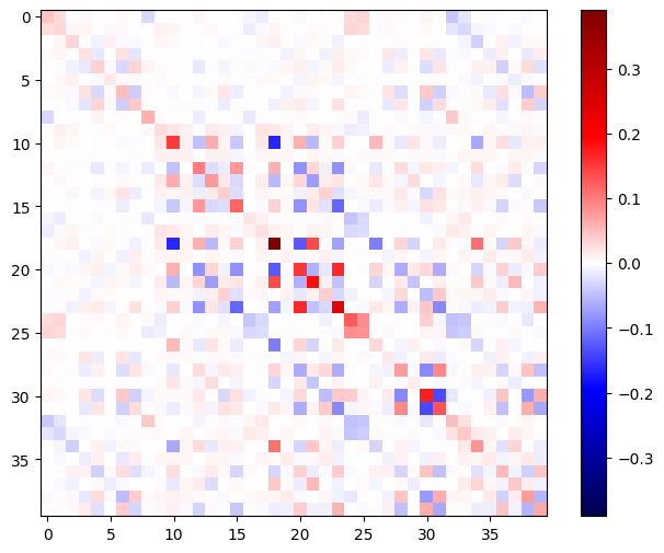
เมทริกซ์เฮสเซียนควรสมมาตร:
def imshow_zero_center(image, **kwargs):
  lim = tf.reduce_max(abs(image))
  plt.imshow(image, vmin=-lim, vmax=lim, cmap='seismic', **kwargs)
  plt.colorbar()
imshow_zero_center(h_mat)
ขั้นตอนการอัปเดตวิธีการของนิวตันแสดงไว้ด้านล่าง:
eps = 1e-3
eye_eps = tf.eye(h_mat.shape[0])*eps
# X(k+1) = X(k) - (∇²f(X(k)))^-1 @ ∇f(X(k))
# h_mat = ∇²f(X(k))
# g_vec = ∇f(X(k))
update = tf.linalg.solve(h_mat + eye_eps, g_vec)

# Reshape the update and apply it to the variable.
_ = layer1.kernel.assign_sub(tf.reshape(update, layer1.kernel.shape))
แม้ว่าสิ่งนี้จะค่อนข้างง่ายสำหรับ tf.Variable ตัวเดียว แต่การนำสิ่งนี้ไปใช้กับโมเดลที่ไม่สำคัญจะต้องมีการต่อและแบ่งอย่างระมัดระวังเพื่อสร้าง Hessian แบบเต็มในหลายตัวแปร
Batch Jacobian
ในบางกรณี คุณต้องการนำจาโคเบียนของเป้าหมายแต่ละกลุ่มโดยเทียบกับกลุ่มแหล่งที่มา โดยที่จาโคเบียนสำหรับคู่เป้าหมาย-แหล่งที่มาแต่ละคู่เป็นอิสระจากกัน
ตัวอย่างเช่น ที่นี่อินพุต x มีรูปร่าง (batch, ins) และเอาต์พุต y มีรูปร่าง (batch, outs) :
x = tf.random.normal([7, 5])

layer1 = tf.keras.layers.Dense(8, activation=tf.nn.elu)
layer2 = tf.keras.layers.Dense(6, activation=tf.nn.elu)

with tf.GradientTape(persistent=True, watch_accessed_variables=False) as tape:
  tape.watch(x)
  y = layer1(x)
  y = layer2(y)

y.shape
TensorShape([7, 6])
Jacobian เต็มรูปแบบของ y เกี่ยวกับ x มีรูปร่างของ (batch, ins, batch, outs) แม้ว่าคุณต้องการเพียง (batch, ins, outs) :
j = tape.jacobian(y, x)
j.shape
TensorShape([7, 6, 7, 5])
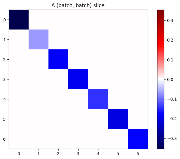
หากการไล่ระดับสีของแต่ละรายการในสแต็กเป็นอิสระ ทุกส่วนของเทนเซอร์นี้ (batch, batch) จะเป็นเมทริกซ์แนวทแยง:
imshow_zero_center(j[:, 0, :, 0])
_ = plt.title('A (batch, batch) slice')
def plot_as_patches(j):
  # Reorder axes so the diagonals will each form a contiguous patch.
  j = tf.transpose(j, [1, 0, 3, 2])
  # Pad in between each patch.
  lim = tf.reduce_max(abs(j))
  j = tf.pad(j, [[0, 0], [1, 1], [0, 0], [1, 1]],
             constant_values=-lim)
  # Reshape to form a single image.
  s = j.shape
  j = tf.reshape(j, [s[0]*s[1], s[2]*s[3]])
  imshow_zero_center(j, extent=[-0.5, s[2]-0.5, s[0]-0.5, -0.5])

plot_as_patches(j)
_ = plt.title('All (batch, batch) slices are diagonal')
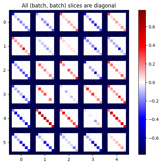
เพื่อให้ได้ผลลัพธ์ที่ต้องการ คุณสามารถรวมมิติ batch งานที่ซ้ำกัน หรือเลือกเส้นทแยงมุมโดยใช้ tf.einsum :
j_sum = tf.reduce_sum(j, axis=2)
print(j_sum.shape)
j_select = tf.einsum('bxby->bxy', j)
print(j_select.shape)
(7, 6, 5)
(7, 6, 5)
ตัวยึดตำแหน่ง51
มันจะมีประสิทธิภาพมากขึ้นในการคำนวณโดยไม่มีมิติพิเศษตั้งแต่แรก วิธี tf.GradientTape.batch_jacobian ทำอย่างนั้น:
jb = tape.batch_jacobian(y, x)
jb.shape
WARNING:tensorflow:5 out of the last 5 calls to <function pfor.<locals>.f at 0x7f7d601250e0> triggered tf.function retracing. Tracing is expensive and the excessive number of tracings could be due to (1) creating @tf.function repeatedly in a loop, (2) passing tensors with different shapes, (3) passing Python objects instead of tensors. For (1), please define your @tf.function outside of the loop. For (2), @tf.function has experimental_relax_shapes=True option that relaxes argument shapes that can avoid unnecessary retracing. For (3), please refer to https://www.tensorflow.org/guide/function#controlling_retracing and https://www.tensorflow.org/api_docs/python/tf/function for  more details.
TensorShape([7, 6, 5])
error = tf.reduce_max(abs(jb - j_sum))
assert error < 1e-3
print(error.numpy())
0.0
x = tf.random.normal([7, 5])

layer1 = tf.keras.layers.Dense(8, activation=tf.nn.elu)
bn = tf.keras.layers.BatchNormalization()
layer2 = tf.keras.layers.Dense(6, activation=tf.nn.elu)

with tf.GradientTape(persistent=True, watch_accessed_variables=False) as tape:
  tape.watch(x)
  y = layer1(x)
  y = bn(y, training=True)
  y = layer2(y)

j = tape.jacobian(y, x)
print(f'j.shape: {j.shape}')
WARNING:tensorflow:6 out of the last 6 calls to <function pfor.<locals>.f at 0x7f7cf062fa70> triggered tf.function retracing. Tracing is expensive and the excessive number of tracings could be due to (1) creating @tf.function repeatedly in a loop, (2) passing tensors with different shapes, (3) passing Python objects instead of tensors. For (1), please define your @tf.function outside of the loop. For (2), @tf.function has experimental_relax_shapes=True option that relaxes argument shapes that can avoid unnecessary retracing. For (3), please refer to https://www.tensorflow.org/guide/function#controlling_retracing and https://www.tensorflow.org/api_docs/python/tf/function for  more details.
j.shape: (7, 6, 7, 5)
plot_as_patches(j)

_ = plt.title('These slices are not diagonal')
_ = plt.xlabel("Don't use `batch_jacobian`")
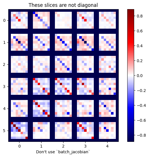
ในกรณีนี้ batch_jacobian ยังคงทำงานและส่งคืน บางสิ่ง ที่มีรูปร่างตามที่คาดไว้ แต่เนื้อหานั้นมีความหมายไม่ชัดเจน:
jb = tape.batch_jacobian(y, x)
print(f'jb.shape: {jb.shape}')
jb.shape: (7, 6, 5)ตัวยึดตำแหน่ง60