
| | |  Visualizza l'origine su GitHub Visualizza l'origine su GitHub | |
Questo tutorial fornisce esempi di come caricare DataFrames Panda in TensorFlow.
Utilizzerai un piccolo set di dati sulle malattie cardiache fornito dall'UCI Machine Learning Repository. Ci sono diverse centinaia di righe nel CSV. Ogni riga descrive un paziente e ogni colonna descrive un attributo. Utilizzerai queste informazioni per prevedere se un paziente ha una malattia cardiaca, che è un'attività di classificazione binaria.
Leggi i dati usando i panda
import pandas as pd
import tensorflow as tf

SHUFFLE_BUFFER = 500
BATCH_SIZE = 2
Scarica il file CSV contenente il dataset delle malattie cardiache:
csv_file = tf.keras.utils.get_file('heart.csv', 'https://storage.googleapis.com/download.tensorflow.org/data/heart.csv')
Downloading data from https://storage.googleapis.com/download.tensorflow.org/data/heart.csv
16384/13273 [=====================================] - 0s 0us/step
24576/13273 [=======================================================] - 0s 0us/step
Leggi il file CSV usando i panda:
df = pd.read_csv(csv_file)
Ecco come appaiono i dati:
df.head()
df.dtypes
age           int64
sex           int64
cp            int64
trestbps      int64
chol          int64
fbs           int64
restecg       int64
thalach       int64
exang         int64
oldpeak     float64
slope         int64
ca            int64
thal         object
target        int64
dtype: object
Creerai modelli per prevedere l'etichetta contenuta nella colonna di target .
target = df.pop('target')
Un DataFrame come array
Se i tuoi dati hanno un tipo di dati uniforme, o dtype , è possibile utilizzare un DataFrame panda ovunque tu possa usare un array NumPy. Funziona perché la classe pandas.DataFrame supporta il protocollo __array__ e la funzione tf.convert_to_tensor di TensorFlow accetta oggetti che supportano il protocollo.
Prendi le funzionalità numeriche dal set di dati (salta le funzionalità categoriali per ora):
numeric_feature_names = ['age', 'thalach', 'trestbps',  'chol', 'oldpeak']
numeric_features = df[numeric_feature_names]
numeric_features.head()
Il DataFrame può essere convertito in una matrice NumPy usando la proprietà DataFrame.values o numpy.array(df) . Per convertirlo in un tensore, usa tf.convert_to_tensor :
tf.convert_to_tensor(numeric_features)
<tf.Tensor: shape=(303, 5), dtype=float64, numpy=
array([[ 63. , 150. , 145. , 233. ,   2.3],
       [ 67. , 108. , 160. , 286. ,   1.5],
       [ 67. , 129. , 120. , 229. ,   2.6],
       ...,
       [ 65. , 127. , 135. , 254. ,   2.8],
       [ 48. , 150. , 130. , 256. ,   0. ],
       [ 63. , 154. , 150. , 407. ,   4. ]])>
In generale, se un oggetto può essere convertito in un tensore con tf.convert_to_tensor , può essere passato ovunque tu possa passare un tf.Tensor .
Con Model.fit
Un DataFrame, interpretato come un singolo tensore, può essere utilizzato direttamente come argomento del metodo Model.fit .
Di seguito è riportato un esempio di addestramento di un modello sulle caratteristiche numeriche del set di dati.
Il primo passo è normalizzare gli intervalli di input. Usa un livello tf.keras.layers.Normalization per quello.
Per impostare la media e la deviazione standard del livello prima di eseguirlo, assicurati di chiamare il metodo Normalization.adapt :
normalizer = tf.keras.layers.Normalization(axis=-1)
normalizer.adapt(numeric_features)
Chiama il livello sulle prime tre righe di DataFrame per visualizzare un esempio dell'output di questo livello:
normalizer(numeric_features.iloc[:3])
<tf.Tensor: shape=(3, 5), dtype=float32, numpy=
array([[ 0.93383914,  0.03480718,  0.74578077, -0.26008663,  1.0680453 ],
       [ 1.3782105 , -1.7806165 ,  1.5923285 ,  0.7573877 ,  0.38022864],
       [ 1.3782105 , -0.87290466, -0.6651321 , -0.33687714,  1.3259765 ]],
      dtype=float32)>
Usa il livello di normalizzazione come primo livello di un modello semplice:
def get_basic_model():
  model = tf.keras.Sequential([
    normalizer,
    tf.keras.layers.Dense(10, activation='relu'),
    tf.keras.layers.Dense(10, activation='relu'),
    tf.keras.layers.Dense(1)
  ])

  model.compile(optimizer='adam',
                loss=tf.keras.losses.BinaryCrossentropy(from_logits=True),
                metrics=['accuracy'])
  return model
Quando si passa DataFrame come argomento x a Model.fit , Keras tratta DataFrame come se fosse un array NumPy:
model = get_basic_model()
model.fit(numeric_features, target, epochs=15, batch_size=BATCH_SIZE)
Epoch 1/15
152/152 [==============================] - 1s 2ms/step - loss: 0.6839 - accuracy: 0.7690
Epoch 2/15
152/152 [==============================] - 0s 2ms/step - loss: 0.5789 - accuracy: 0.7789
Epoch 3/15
152/152 [==============================] - 0s 2ms/step - loss: 0.5195 - accuracy: 0.7723
Epoch 4/15
152/152 [==============================] - 0s 2ms/step - loss: 0.4814 - accuracy: 0.7855
Epoch 5/15
152/152 [==============================] - 0s 2ms/step - loss: 0.4566 - accuracy: 0.7789
Epoch 6/15
152/152 [==============================] - 0s 2ms/step - loss: 0.4427 - accuracy: 0.7888
Epoch 7/15
152/152 [==============================] - 0s 2ms/step - loss: 0.4342 - accuracy: 0.7921
Epoch 8/15
152/152 [==============================] - 0s 2ms/step - loss: 0.4290 - accuracy: 0.7855
Epoch 9/15
152/152 [==============================] - 0s 2ms/step - loss: 0.4240 - accuracy: 0.7987
Epoch 10/15
152/152 [==============================] - 0s 2ms/step - loss: 0.4232 - accuracy: 0.7987
Epoch 11/15
152/152 [==============================] - 0s 2ms/step - loss: 0.4208 - accuracy: 0.7987
Epoch 12/15
152/152 [==============================] - 0s 2ms/step - loss: 0.4186 - accuracy: 0.7954
Epoch 13/15
152/152 [==============================] - 0s 2ms/step - loss: 0.4172 - accuracy: 0.8020
Epoch 14/15
152/152 [==============================] - 0s 2ms/step - loss: 0.4156 - accuracy: 0.8020
Epoch 15/15
152/152 [==============================] - 0s 2ms/step - loss: 0.4138 - accuracy: 0.8020
<keras.callbacks.History at 0x7f1ddc27b110>
Con tf.data
Se vuoi applicare le trasformazioni tf.data a un DataFrame di un uniforme dtype , il metodo Dataset.from_tensor_slices creerà un set di dati che scorre sulle righe di DataFrame. Ogni riga è inizialmente un vettore di valori. Per addestrare un modello, sono necessarie coppie (inputs, labels) , quindi pass (features, labels) e Dataset.from_tensor_slices restituiranno le coppie di slice necessarie:
numeric_dataset = tf.data.Dataset.from_tensor_slices((numeric_features, target))

for row in numeric_dataset.take(3):
  print(row)
(<tf.Tensor: shape=(5,), dtype=float64, numpy=array([ 63. , 150. , 145. , 233. ,   2.3])>, <tf.Tensor: shape=(), dtype=int64, numpy=0>)
(<tf.Tensor: shape=(5,), dtype=float64, numpy=array([ 67. , 108. , 160. , 286. ,   1.5])>, <tf.Tensor: shape=(), dtype=int64, numpy=1>)
(<tf.Tensor: shape=(5,), dtype=float64, numpy=array([ 67. , 129. , 120. , 229. ,   2.6])>, <tf.Tensor: shape=(), dtype=int64, numpy=0>)
numeric_batches = numeric_dataset.shuffle(1000).batch(BATCH_SIZE)

model = get_basic_model()
model.fit(numeric_batches, epochs=15)
Epoch 1/15
152/152 [==============================] - 1s 2ms/step - loss: 0.7677 - accuracy: 0.6865
Epoch 2/15
152/152 [==============================] - 0s 2ms/step - loss: 0.6319 - accuracy: 0.7591
Epoch 3/15
152/152 [==============================] - 0s 2ms/step - loss: 0.5717 - accuracy: 0.7459
Epoch 4/15
152/152 [==============================] - 0s 2ms/step - loss: 0.5228 - accuracy: 0.7558
Epoch 5/15
152/152 [==============================] - 0s 2ms/step - loss: 0.4820 - accuracy: 0.7624
Epoch 6/15
152/152 [==============================] - 0s 2ms/step - loss: 0.4584 - accuracy: 0.7657
Epoch 7/15
152/152 [==============================] - 0s 2ms/step - loss: 0.4454 - accuracy: 0.7657
Epoch 8/15
152/152 [==============================] - 0s 2ms/step - loss: 0.4379 - accuracy: 0.7789
Epoch 9/15
152/152 [==============================] - 0s 2ms/step - loss: 0.4324 - accuracy: 0.7789
Epoch 10/15
152/152 [==============================] - 0s 2ms/step - loss: 0.4282 - accuracy: 0.7756
Epoch 11/15
152/152 [==============================] - 0s 2ms/step - loss: 0.4273 - accuracy: 0.7789
Epoch 12/15
152/152 [==============================] - 0s 2ms/step - loss: 0.4268 - accuracy: 0.7756
Epoch 13/15
152/152 [==============================] - 0s 2ms/step - loss: 0.4248 - accuracy: 0.7789
Epoch 14/15
152/152 [==============================] - 0s 2ms/step - loss: 0.4235 - accuracy: 0.7855
Epoch 15/15
152/152 [==============================] - 0s 2ms/step - loss: 0.4223 - accuracy: 0.7888
<keras.callbacks.History at 0x7f1ddc406510>
Un DataFrame come dizionario
Quando inizi a gestire dati eterogenei, non è più possibile trattare DataFrame come se fosse un singolo array. I tensori TensorFlow richiedono che tutti gli elementi abbiano lo stesso dtype .
Quindi, in questo caso, devi iniziare a trattarlo come un dizionario di colonne, dove ogni colonna ha un dtype uniforme. Un DataFrame è molto simile a un dizionario di array, quindi in genere tutto ciò che devi fare è eseguire il cast di DataFrame su un dict Python. Molte importanti API di TensorFlow supportano dizionari (nidificati) di array come input.
Le pipeline di input tf.data gestiscono abbastanza bene. Tutte le operazioni tf.data gestiscono automaticamente dizionari e tuple. Quindi, per creare un set di dati di esempi di dizionario da un DataFrame, basta eseguirne il cast su un dict prima di tagliarlo con Dataset.from_tensor_slices :
numeric_dict_ds = tf.data.Dataset.from_tensor_slices((dict(numeric_features), target))
Ecco i primi tre esempi di quel set di dati:
for row in numeric_dict_ds.take(3):
  print(row)
({'age': <tf.Tensor: shape=(), dtype=int64, numpy=63>, 'thalach': <tf.Tensor: shape=(), dtype=int64, numpy=150>, 'trestbps': <tf.Tensor: shape=(), dtype=int64, numpy=145>, 'chol': <tf.Tensor: shape=(), dtype=int64, numpy=233>, 'oldpeak': <tf.Tensor: shape=(), dtype=float64, numpy=2.3>}, <tf.Tensor: shape=(), dtype=int64, numpy=0>)
({'age': <tf.Tensor: shape=(), dtype=int64, numpy=67>, 'thalach': <tf.Tensor: shape=(), dtype=int64, numpy=108>, 'trestbps': <tf.Tensor: shape=(), dtype=int64, numpy=160>, 'chol': <tf.Tensor: shape=(), dtype=int64, numpy=286>, 'oldpeak': <tf.Tensor: shape=(), dtype=float64, numpy=1.5>}, <tf.Tensor: shape=(), dtype=int64, numpy=1>)
({'age': <tf.Tensor: shape=(), dtype=int64, numpy=67>, 'thalach': <tf.Tensor: shape=(), dtype=int64, numpy=129>, 'trestbps': <tf.Tensor: shape=(), dtype=int64, numpy=120>, 'chol': <tf.Tensor: shape=(), dtype=int64, numpy=229>, 'oldpeak': <tf.Tensor: shape=(), dtype=float64, numpy=2.6>}, <tf.Tensor: shape=(), dtype=int64, numpy=0>)
Dizionari con Keras
Tipicamente, i modelli e i livelli Keras prevedono un singolo tensore di input, ma queste classi possono accettare e restituire strutture nidificate di dizionari, tuple e tensori. Queste strutture sono conosciute come "nidi" (fare riferimento al modulo tf.nest per i dettagli).
Esistono due modi equivalenti per scrivere un modello keras che accetta un dizionario come input.
1. Lo stile della sottoclasse Modello
Scrivi una sottoclasse di tf.keras.Model (o tf.keras.Layer ). Gestisci direttamente gli input e crei gli output:
def stack_dict(inputs, fun=tf.stack):
    values = []
    for key in sorted(inputs.keys()):
      values.append(tf.cast(inputs[key], tf.float32))

    return fun(values, axis=-1)
class MyModel(tf.keras.Model):
  def __init__(self):
    # Create all the internal layers in init.
    super().__init__(self)

    self.normalizer = tf.keras.layers.Normalization(axis=-1)

    self.seq = tf.keras.Sequential([
      self.normalizer,
      tf.keras.layers.Dense(10, activation='relu'),
      tf.keras.layers.Dense(10, activation='relu'),
      tf.keras.layers.Dense(1)
    ])

  def adapt(self, inputs):
    # Stach the inputs and `adapt` the normalization layer.
    inputs = stack_dict(inputs)
    self.normalizer.adapt(inputs)

  def call(self, inputs):
    # Stack the inputs
    inputs = stack_dict(inputs)
    # Run them through all the layers.
    result = self.seq(inputs)

    return result

model = MyModel()

model.adapt(dict(numeric_features))

model.compile(optimizer='adam',
              loss=tf.keras.losses.BinaryCrossentropy(from_logits=True),
              metrics=['accuracy'],
              run_eagerly=True)
Questo modello può accettare un dizionario di colonne o un set di dati di elementi dizionario per l'addestramento:
model.fit(dict(numeric_features), target, epochs=5, batch_size=BATCH_SIZE)
Epoch 1/5
152/152 [==============================] - 3s 17ms/step - loss: 0.6736 - accuracy: 0.7063
Epoch 2/5
152/152 [==============================] - 3s 17ms/step - loss: 0.5577 - accuracy: 0.7294
Epoch 3/5
152/152 [==============================] - 2s 16ms/step - loss: 0.4869 - accuracy: 0.7591
Epoch 4/5
152/152 [==============================] - 2s 16ms/step - loss: 0.4525 - accuracy: 0.7690
Epoch 5/5
152/152 [==============================] - 2s 16ms/step - loss: 0.4403 - accuracy: 0.7624
<keras.callbacks.History at 0x7f1de4fa9390>
numeric_dict_batches = numeric_dict_ds.shuffle(SHUFFLE_BUFFER).batch(BATCH_SIZE)
model.fit(numeric_dict_batches, epochs=5)
Epoch 1/5
152/152 [==============================] - 2s 15ms/step - loss: 0.4328 - accuracy: 0.7756
Epoch 2/5
152/152 [==============================] - 2s 14ms/step - loss: 0.4297 - accuracy: 0.7888
Epoch 3/5
152/152 [==============================] - 2s 15ms/step - loss: 0.4270 - accuracy: 0.7888
Epoch 4/5
152/152 [==============================] - 2s 15ms/step - loss: 0.4245 - accuracy: 0.8020
Epoch 5/5
152/152 [==============================] - 2s 15ms/step - loss: 0.4240 - accuracy: 0.7921
<keras.callbacks.History at 0x7f1ddc0dba90>
Ecco le previsioni per i primi tre esempi:
model.predict(dict(numeric_features.iloc[:3]))
array([[[0.00565109]],

       [[0.60601974]],

       [[0.03647463]]], dtype=float32)
2. Lo stile funzionale Keras
inputs = {}
for name, column in numeric_features.items():
  inputs[name] = tf.keras.Input(
      shape=(1,), name=name, dtype=tf.float32)

inputs
{'age': <KerasTensor: shape=(None, 1) dtype=float32 (created by layer 'age')>,
 'thalach': <KerasTensor: shape=(None, 1) dtype=float32 (created by layer 'thalach')>,
 'trestbps': <KerasTensor: shape=(None, 1) dtype=float32 (created by layer 'trestbps')>,
 'chol': <KerasTensor: shape=(None, 1) dtype=float32 (created by layer 'chol')>,
 'oldpeak': <KerasTensor: shape=(None, 1) dtype=float32 (created by layer 'oldpeak')>}
x = stack_dict(inputs, fun=tf.concat)

normalizer = tf.keras.layers.Normalization(axis=-1)
normalizer.adapt(stack_dict(dict(numeric_features)))

x = normalizer(x)
x = tf.keras.layers.Dense(10, activation='relu')(x)
x = tf.keras.layers.Dense(10, activation='relu')(x)
x = tf.keras.layers.Dense(1)(x)

model = tf.keras.Model(inputs, x)

model.compile(optimizer='adam',
              loss=tf.keras.losses.BinaryCrossentropy(from_logits=True),
              metrics=['accuracy'],
              run_eagerly=True)
tf.keras.utils.plot_model(model, rankdir="LR", show_shapes=True)
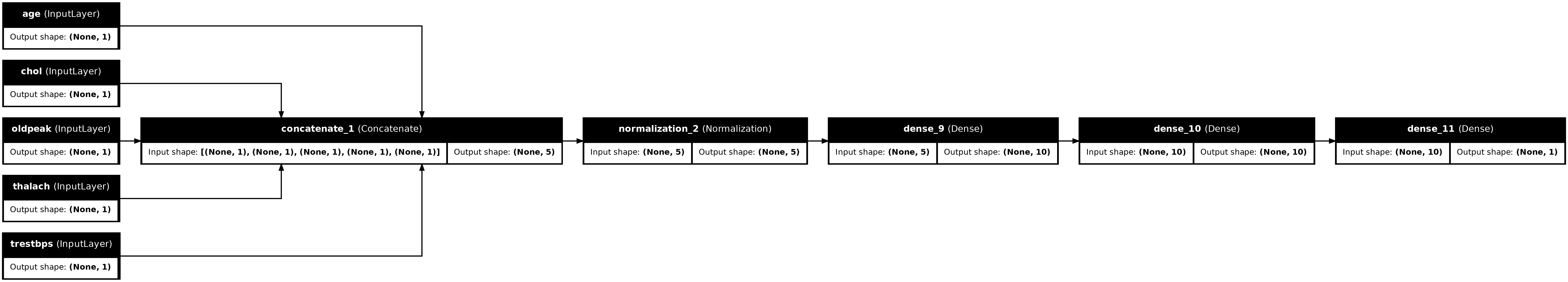
Puoi addestrare il modello funzionale allo stesso modo della sottoclasse del modello:
model.fit(dict(numeric_features), target, epochs=5, batch_size=BATCH_SIZE)
Epoch 1/5
152/152 [==============================] - 2s 15ms/step - loss: 0.6529 - accuracy: 0.7492
Epoch 2/5
152/152 [==============================] - 2s 15ms/step - loss: 0.5448 - accuracy: 0.7624
Epoch 3/5
152/152 [==============================] - 2s 15ms/step - loss: 0.4935 - accuracy: 0.7756
Epoch 4/5
152/152 [==============================] - 2s 15ms/step - loss: 0.4650 - accuracy: 0.7789
Epoch 5/5
152/152 [==============================] - 2s 15ms/step - loss: 0.4486 - accuracy: 0.7855
<keras.callbacks.History at 0x7f1ddc0d0f90>
numeric_dict_batches = numeric_dict_ds.shuffle(SHUFFLE_BUFFER).batch(BATCH_SIZE)
model.fit(numeric_dict_batches, epochs=5)
Epoch 1/5
152/152 [==============================] - 2s 15ms/step - loss: 0.4398 - accuracy: 0.7855
Epoch 2/5
152/152 [==============================] - 2s 15ms/step - loss: 0.4330 - accuracy: 0.7855
Epoch 3/5
152/152 [==============================] - 2s 16ms/step - loss: 0.4294 - accuracy: 0.7921
Epoch 4/5
152/152 [==============================] - 2s 16ms/step - loss: 0.4271 - accuracy: 0.7888
Epoch 5/5
152/152 [==============================] - 2s 16ms/step - loss: 0.4231 - accuracy: 0.7855
<keras.callbacks.History at 0x7f1d7c5d5d10>
Esempio completo
Se stai passando un DataFrame eterogeneo a Keras, ogni colonna potrebbe richiedere una preelaborazione univoca. È possibile eseguire questa preelaborazione direttamente in DataFrame, ma affinché un modello funzioni correttamente, gli input devono sempre essere preelaborati allo stesso modo. Quindi, l'approccio migliore è costruire la preelaborazione nel modello. I livelli di preelaborazione di Keras coprono molte attività comuni.
Costruisci la testa di preelaborazione
In questo set di dati alcune delle caratteristiche "intere" nei dati grezzi sono in realtà indici categoriali. Questi indici non sono valori numerici realmente ordinati (fare riferimento alla descrizione del set di dati per i dettagli). Poiché questi non sono ordinati, sono inadeguati da alimentare direttamente al modello; il modello li interpreterebbe come ordinati. Per utilizzare questi input dovrai codificarli, come vettori one-hot o come vettori di incorporamento. Lo stesso vale per le caratteristiche di categoria stringa.
Le caratteristiche binarie d'altra parte generalmente non hanno bisogno di essere codificate o normalizzate.
Inizia creando un elenco delle funzionalità che rientrano in ciascun gruppo:
binary_feature_names = ['sex', 'fbs', 'exang']
categorical_feature_names = ['cp', 'restecg', 'slope', 'thal', 'ca']
Il passaggio successivo consiste nel creare un modello di preelaborazione che applichi la preelaborazione appropriata a ciascuno di ciascun input e concateni i risultati.
Questa sezione utilizza l' API funzionale Keras per implementare la preelaborazione. Inizi creando un tf.keras.Input per ogni colonna del dataframe:
inputs = {}
for name, column in df.items():
  if type(column[0]) == str:
    dtype = tf.string
  elif (name in categorical_feature_names or
        name in binary_feature_names):
    dtype = tf.int64
  else:
    dtype = tf.float32

  inputs[name] = tf.keras.Input(shape=(), name=name, dtype=dtype)
inputs
{'age': <KerasTensor: shape=(None,) dtype=float32 (created by layer 'age')>,
 'sex': <KerasTensor: shape=(None,) dtype=int64 (created by layer 'sex')>,
 'cp': <KerasTensor: shape=(None,) dtype=int64 (created by layer 'cp')>,
 'trestbps': <KerasTensor: shape=(None,) dtype=float32 (created by layer 'trestbps')>,
 'chol': <KerasTensor: shape=(None,) dtype=float32 (created by layer 'chol')>,
 'fbs': <KerasTensor: shape=(None,) dtype=int64 (created by layer 'fbs')>,
 'restecg': <KerasTensor: shape=(None,) dtype=int64 (created by layer 'restecg')>,
 'thalach': <KerasTensor: shape=(None,) dtype=float32 (created by layer 'thalach')>,
 'exang': <KerasTensor: shape=(None,) dtype=int64 (created by layer 'exang')>,
 'oldpeak': <KerasTensor: shape=(None,) dtype=float32 (created by layer 'oldpeak')>,
 'slope': <KerasTensor: shape=(None,) dtype=int64 (created by layer 'slope')>,
 'ca': <KerasTensor: shape=(None,) dtype=int64 (created by layer 'ca')>,
 'thal': <KerasTensor: shape=(None,) dtype=string (created by layer 'thal')>}
Per ogni input applicherai alcune trasformazioni usando i livelli Keras e le operazioni TensorFlow. Ogni funzionalità inizia come un batch di scalari ( shape=(batch,) ). L'output per ciascuno dovrebbe essere un batch di vettori tf.float32 ( shape=(batch, n) ). L'ultimo passaggio concatenerà tutti quei vettori insieme.
Ingressi binari
Poiché gli input binari non necessitano di alcuna preelaborazione, basta aggiungere l'asse vettoriale, eseguirne il cast su float32 e aggiungerli all'elenco degli input preelaborati:
preprocessed = []

for name in binary_feature_names:
  inp = inputs[name]
  inp = inp[:, tf.newaxis]
  float_value = tf.cast(inp, tf.float32)
  preprocessed.append(float_value)

preprocessed
[<KerasTensor: shape=(None, 1) dtype=float32 (created by layer 'tf.cast_5')>,
 <KerasTensor: shape=(None, 1) dtype=float32 (created by layer 'tf.cast_6')>,
 <KerasTensor: shape=(None, 1) dtype=float32 (created by layer 'tf.cast_7')>]
Ingressi numerici
Come nella sezione precedente, ti consigliamo di eseguire questi input numerici attraverso un livello tf.keras.layers.Normalization prima di usarli. La differenza è che questa volta vengono inseriti come dict. Il codice seguente raccoglie le funzionalità numeriche da DataFrame, le impila insieme e le passa al metodo Normalization.adapt .
normalizer = tf.keras.layers.Normalization(axis=-1)
normalizer.adapt(stack_dict(dict(numeric_features)))
Il codice seguente impila le funzionalità numeriche e le esegue attraverso il livello di normalizzazione.
numeric_inputs = {}
for name in numeric_feature_names:
  numeric_inputs[name]=inputs[name]

numeric_inputs = stack_dict(numeric_inputs)
numeric_normalized = normalizer(numeric_inputs)

preprocessed.append(numeric_normalized)

preprocessed
[<KerasTensor: shape=(None, 1) dtype=float32 (created by layer 'tf.cast_5')>,
 <KerasTensor: shape=(None, 1) dtype=float32 (created by layer 'tf.cast_6')>,
 <KerasTensor: shape=(None, 1) dtype=float32 (created by layer 'tf.cast_7')>,
 <KerasTensor: shape=(None, 5) dtype=float32 (created by layer 'normalization_3')>]
Caratteristiche categoriali
Per utilizzare le funzionalità categoriali devi prima codificarle in vettori binari o incorporamenti. Poiché queste funzionalità contengono solo un numero limitato di categorie, converti gli input direttamente in vettori one-hot utilizzando l' output_mode='one_hot' , supportata da entrambi i tf.keras.layers.StringLookup e tf.keras.layers.IntegerLookup .
Ecco un esempio di come funzionano questi livelli:
vocab = ['a','b','c']
lookup = tf.keras.layers.StringLookup(vocabulary=vocab, output_mode='one_hot')
lookup(['c','a','a','b','zzz'])
<tf.Tensor: shape=(5, 4), dtype=float32, numpy=
array([[0., 0., 0., 1.],
       [0., 1., 0., 0.],
       [0., 1., 0., 0.],
       [0., 0., 1., 0.],
       [1., 0., 0., 0.]], dtype=float32)>
vocab = [1,4,7,99]
lookup = tf.keras.layers.IntegerLookup(vocabulary=vocab, output_mode='one_hot')

lookup([-1,4,1])
<tf.Tensor: shape=(3, 5), dtype=float32, numpy=
array([[1., 0., 0., 0., 0.],
       [0., 0., 1., 0., 0.],
       [0., 1., 0., 0., 0.]], dtype=float32)>
Per determinare il vocabolario per ogni input, crea un livello per convertire quel vocabolario in un vettore one-hot:
for name in categorical_feature_names:
  vocab = sorted(set(df[name]))
  print(f'name: {name}')
  print(f'vocab: {vocab}\n')

  if type(vocab[0]) is str:
    lookup = tf.keras.layers.StringLookup(vocabulary=vocab, output_mode='one_hot')
  else:
    lookup = tf.keras.layers.IntegerLookup(vocabulary=vocab, output_mode='one_hot')

  x = inputs[name][:, tf.newaxis]
  x = lookup(x)
  preprocessed.append(x)
name: cp
vocab: [0, 1, 2, 3, 4]

name: restecg
vocab: [0, 1, 2]

name: slope
vocab: [1, 2, 3]

name: thal
vocab: ['1', '2', 'fixed', 'normal', 'reversible']

name: ca
vocab: [0, 1, 2, 3]
Montare la testa di preelaborazione
A questo punto preprocessed è solo un elenco Python di tutti i risultati di preelaborazione, ogni risultato ha una forma di (batch_size, depth) :
preprocessed
[<KerasTensor: shape=(None, 1) dtype=float32 (created by layer 'tf.cast_5')>,
 <KerasTensor: shape=(None, 1) dtype=float32 (created by layer 'tf.cast_6')>,
 <KerasTensor: shape=(None, 1) dtype=float32 (created by layer 'tf.cast_7')>,
 <KerasTensor: shape=(None, 5) dtype=float32 (created by layer 'normalization_3')>,
 <KerasTensor: shape=(None, 6) dtype=float32 (created by layer 'integer_lookup_1')>,
 <KerasTensor: shape=(None, 4) dtype=float32 (created by layer 'integer_lookup_2')>,
 <KerasTensor: shape=(None, 4) dtype=float32 (created by layer 'integer_lookup_3')>,
 <KerasTensor: shape=(None, 6) dtype=float32 (created by layer 'string_lookup_1')>,
 <KerasTensor: shape=(None, 5) dtype=float32 (created by layer 'integer_lookup_4')>]
Concatena tutte le funzioni preelaborate lungo l'asse di depth , in modo che ogni esempio di dizionario venga convertito in un unico vettore. Il vettore contiene funzionalità categoriali, funzionalità numeriche e funzionalità one-hot categoriali:
preprocesssed_result = tf.concat(preprocessed, axis=-1)
preprocesssed_result
<KerasTensor: shape=(None, 33) dtype=float32 (created by layer 'tf.concat_1')>
Ora crea un modello da quel calcolo in modo che possa essere riutilizzato:
preprocessor = tf.keras.Model(inputs, preprocesssed_result)
tf.keras.utils.plot_model(preprocessor, rankdir="LR", show_shapes=True)
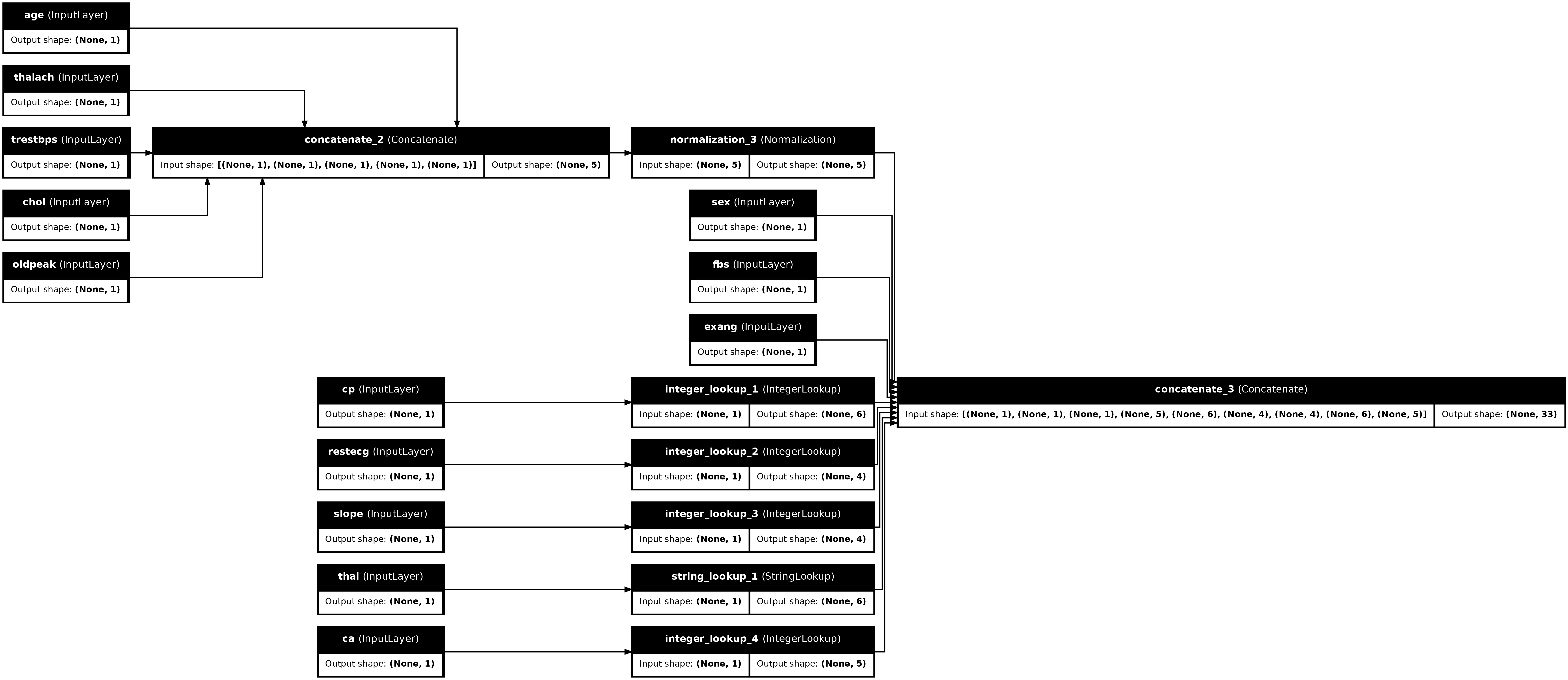
Per testare il preprocessore, usa la funzione di accesso DataFrame.iloc per dividere il primo esempio da DataFrame. Quindi convertilo in un dizionario e passa il dizionario al preprocessore. Il risultato è un singolo vettore contenente le caratteristiche binarie, le caratteristiche numeriche normalizzate e le caratteristiche categoriali one-hot, in quest'ordine:
preprocessor(dict(df.iloc[:1]))
<tf.Tensor: shape=(1, 33), dtype=float32, numpy=
array([[ 1.        ,  1.        ,  0.        ,  0.93383914, -0.26008663,
         1.0680453 ,  0.03480718,  0.74578077,  0.        ,  0.        ,

         1.        ,  0.        ,  0.        ,  0.        ,  0.        ,
         0.        ,  0.        ,  1.        ,  0.        ,  0.        ,
         0.        ,  1.        ,  0.        ,  0.        ,  0.        ,
         1.        ,  0.        ,  0.        ,  0.        ,  1.        ,
         0.        ,  0.        ,  0.        ]], dtype=float32)>
Crea e addestra un modello
Ora costruisci il corpo principale del modello. Utilizzare la stessa configurazione dell'esempio precedente: un paio di strati lineari rettificati Dense e uno strato di output Dense(1) per la classificazione.
body = tf.keras.Sequential([
  tf.keras.layers.Dense(10, activation='relu'),
  tf.keras.layers.Dense(10, activation='relu'),
  tf.keras.layers.Dense(1)
])
Ora metti insieme i due pezzi usando l'API funzionale di Keras.
inputs
{'age': <KerasTensor: shape=(None,) dtype=float32 (created by layer 'age')>,
 'sex': <KerasTensor: shape=(None,) dtype=int64 (created by layer 'sex')>,
 'cp': <KerasTensor: shape=(None,) dtype=int64 (created by layer 'cp')>,
 'trestbps': <KerasTensor: shape=(None,) dtype=float32 (created by layer 'trestbps')>,
 'chol': <KerasTensor: shape=(None,) dtype=float32 (created by layer 'chol')>,
 'fbs': <KerasTensor: shape=(None,) dtype=int64 (created by layer 'fbs')>,
 'restecg': <KerasTensor: shape=(None,) dtype=int64 (created by layer 'restecg')>,
 'thalach': <KerasTensor: shape=(None,) dtype=float32 (created by layer 'thalach')>,
 'exang': <KerasTensor: shape=(None,) dtype=int64 (created by layer 'exang')>,
 'oldpeak': <KerasTensor: shape=(None,) dtype=float32 (created by layer 'oldpeak')>,
 'slope': <KerasTensor: shape=(None,) dtype=int64 (created by layer 'slope')>,
 'ca': <KerasTensor: shape=(None,) dtype=int64 (created by layer 'ca')>,
 'thal': <KerasTensor: shape=(None,) dtype=string (created by layer 'thal')>}
x = preprocessor(inputs)
x
<KerasTensor: shape=(None, 33) dtype=float32 (created by layer 'model_1')>
result = body(x)
result
<KerasTensor: shape=(None, 1) dtype=float32 (created by layer 'sequential_3')>
model = tf.keras.Model(inputs, result)

model.compile(optimizer='adam',
                loss=tf.keras.losses.BinaryCrossentropy(from_logits=True),
                metrics=['accuracy'])
Questo modello prevede un dizionario di input. Il modo più semplice per passargli i dati è convertire DataFrame in un dict e passare quel dict come argomento x a Model.fit :
history = model.fit(dict(df), target, epochs=5, batch_size=BATCH_SIZE)
Epoch 1/5
152/152 [==============================] - 1s 4ms/step - loss: 0.6911 - accuracy: 0.6997
Epoch 2/5
152/152 [==============================] - 1s 4ms/step - loss: 0.5073 - accuracy: 0.7393
Epoch 3/5
152/152 [==============================] - 1s 4ms/step - loss: 0.4129 - accuracy: 0.7888
Epoch 4/5
152/152 [==============================] - 1s 4ms/step - loss: 0.3663 - accuracy: 0.7921
Epoch 5/5
152/152 [==============================] - 1s 4ms/step - loss: 0.3363 - accuracy: 0.8152
Anche l'uso tf.data funziona:
ds = tf.data.Dataset.from_tensor_slices((
    dict(df),
    target
))

ds = ds.batch(BATCH_SIZE)
import pprint

for x, y in ds.take(1):
  pprint.pprint(x)
  print()
  print(y)
{'age': <tf.Tensor: shape=(2,), dtype=int64, numpy=array([63, 67])>,
 'ca': <tf.Tensor: shape=(2,), dtype=int64, numpy=array([0, 3])>,
 'chol': <tf.Tensor: shape=(2,), dtype=int64, numpy=array([233, 286])>,
 'cp': <tf.Tensor: shape=(2,), dtype=int64, numpy=array([1, 4])>,
 'exang': <tf.Tensor: shape=(2,), dtype=int64, numpy=array([0, 1])>,
 'fbs': <tf.Tensor: shape=(2,), dtype=int64, numpy=array([1, 0])>,
 'oldpeak': <tf.Tensor: shape=(2,), dtype=float64, numpy=array([2.3, 1.5])>,
 'restecg': <tf.Tensor: shape=(2,), dtype=int64, numpy=array([2, 2])>,
 'sex': <tf.Tensor: shape=(2,), dtype=int64, numpy=array([1, 1])>,
 'slope': <tf.Tensor: shape=(2,), dtype=int64, numpy=array([3, 2])>,
 'thal': <tf.Tensor: shape=(2,), dtype=string, numpy=array([b'fixed', b'normal'], dtype=object)>,
 'thalach': <tf.Tensor: shape=(2,), dtype=int64, numpy=array([150, 108])>,
 'trestbps': <tf.Tensor: shape=(2,), dtype=int64, numpy=array([145, 160])>}

tf.Tensor([0 1], shape=(2,), dtype=int64)
history = model.fit(ds, epochs=5)
Epoch 1/5
152/152 [==============================] - 1s 5ms/step - loss: 0.3150 - accuracy: 0.8284
Epoch 2/5
152/152 [==============================] - 1s 5ms/step - loss: 0.2989 - accuracy: 0.8449
Epoch 3/5
152/152 [==============================] - 1s 5ms/step - loss: 0.2870 - accuracy: 0.8449
Epoch 4/5
152/152 [==============================] - 1s 5ms/step - loss: 0.2782 - accuracy: 0.8482
Epoch 5/5
152/152 [==============================] - 1s 5ms/step - loss: 0.2712 - accuracy: 0.8482