
| | |  در GitHub مشاهده کنید در GitHub مشاهده کنید | | |
این بررسی طبقه بندی نوت بوک فیلم به عنوان مثبت یا منفی با استفاده از متن نظر. این یک نمونه از باینری -یا دو طبقه-طبقه بندی، نوع مهم و به طور گسترده ای قابل اجرا از مشکل یادگیری ماشین است.
ما در بر خواهید استفاده کنید مجموعه داده IMDB که حاوی متن 50،000 بررسی فیلم از بانک اطلاعات اینترنتی فیلمها . اینها به 25000 بررسی برای آموزش و 25000 بررسی برای آزمایش تقسیم می شوند. مجموعه آموزش و تست متعادل، بدین معنی که شامل تعداد مساوی از بررسی مثبت و منفی.
این نوت بوک با استفاده tf.keras ، یک API سطح بالا به مدل های ساخت و قطار در TensorFlow و TensorFlow توپی ، یک کتابخانه و پلت فرم برای یادگیری انتقال. برای یک متن پیشرفته تر طبقه بندی آموزش استفاده از tf.keras ، را ببینید MLCC متن طبقه بندی راهنمای .
مدل های بیشتر
در اینجا شما می توانید مدل رسا تر و یا سازگار که شما می توانید به تولید تعبیه متن استفاده کنید.
برپایی
import numpy as np

import tensorflow as tf
import tensorflow_hub as hub
import tensorflow_datasets as tfds

import matplotlib.pyplot as plt

print("Version: ", tf.__version__)
print("Eager mode: ", tf.executing_eagerly())
print("Hub version: ", hub.__version__)
print("GPU is", "available" if tf.config.list_physical_devices('GPU') else "NOT AVAILABLE")
Version:  2.7.0
Eager mode:  True
Hub version:  0.12.0
GPU is available
مجموعه داده های IMDB را دانلود کنید
مجموعه داده IMDB در دسترس است مجموعه داده TensorFlow . کد زیر مجموعه داده های IMDB را در دستگاه شما (یا زمان اجرا colab) دانلود می کند:
train_data, test_data = tfds.load(name="imdb_reviews", split=["train", "test"],
                                  batch_size=-1, as_supervised=True)

train_examples, train_labels = tfds.as_numpy(train_data)
test_examples, test_labels = tfds.as_numpy(test_data)
WARNING:tensorflow:From /tmpfs/src/tf_docs_env/lib/python3.7/site-packages/tensorflow_datasets/core/dataset_builder.py:622: get_single_element (from tensorflow.python.data.experimental.ops.get_single_element) is deprecated and will be removed in a future version.
Instructions for updating:
Use `tf.data.Dataset.get_single_element()`.
داده ها را کاوش کنید
بیایید یک لحظه برای درک قالب داده ها وقت بگذاریم. هر مثال یک جمله است که نشان دهنده نقد فیلم و یک برچسب مربوطه است. جمله به هیچ وجه پیش پردازش نشده است. برچسب یک مقدار صحیح 0 یا 1 است که 0 یک بررسی منفی و 1 یک بررسی مثبت است.
print("Training entries: {}, test entries: {}".format(len(train_examples), len(test_examples)))
Training entries: 25000, test entries: 25000
بیایید 10 نمونه اول را چاپ کنیم.
train_examples[:10]
array([b"This was an absolutely terrible movie. Don't be lured in by Christopher Walken or Michael Ironside. Both are great actors, but this must simply be their worst role in history. Even their great acting could not redeem this movie's ridiculous storyline. This movie is an early nineties US propaganda piece. The most pathetic scenes were those when the Columbian rebels were making their cases for revolutions. Maria Conchita Alonso appeared phony, and her pseudo-love affair with Walken was nothing but a pathetic emotional plug in a movie that was devoid of any real meaning. I am disappointed that there are movies like this, ruining actor's like Christopher Walken's good name. I could barely sit through it.",
       b'I have been known to fall asleep during films, but this is usually due to a combination of things including, really tired, being warm and comfortable on the sette and having just eaten a lot. However on this occasion I fell asleep because the film was rubbish. The plot development was constant. Constantly slow and boring. Things seemed to happen, but with no explanation of what was causing them or why. I admit, I may have missed part of the film, but i watched the majority of it and everything just seemed to happen of its own accord without any real concern for anything else. I cant recommend this film at all.',
       b'Mann photographs the Alberta Rocky Mountains in a superb fashion, and Jimmy Stewart and Walter Brennan give enjoyable performances as they always seem to do. <br /><br />But come on Hollywood - a Mountie telling the people of Dawson City, Yukon to elect themselves a marshal (yes a marshal!) and to enforce the law themselves, then gunfighters battling it out on the streets for control of the town? <br /><br />Nothing even remotely resembling that happened on the Canadian side of the border during the Klondike gold rush. Mr. Mann and company appear to have mistaken Dawson City for Deadwood, the Canadian North for the American Wild West.<br /><br />Canadian viewers be prepared for a Reefer Madness type of enjoyable howl with this ludicrous plot, or, to shake your head in disgust.',
       b'This is the kind of film for a snowy Sunday afternoon when the rest of the world can go ahead with its own business as you descend into a big arm-chair and mellow for a couple of hours. Wonderful performances from Cher and Nicolas Cage (as always) gently row the plot along. There are no rapids to cross, no dangerous waters, just a warm and witty paddle through New York life at its best. A family film in every sense and one that deserves the praise it received.',
       b'As others have mentioned, all the women that go nude in this film are mostly absolutely gorgeous. The plot very ably shows the hypocrisy of the female libido. When men are around they want to be pursued, but when no "men" are around, they become the pursuers of a 14 year old boy. And the boy becomes a man really fast (we should all be so lucky at this age!). He then gets up the courage to pursue his true love.',
       b"This is a film which should be seen by anybody interested in, effected by, or suffering from an eating disorder. It is an amazingly accurate and sensitive portrayal of bulimia in a teenage girl, its causes and its symptoms. The girl is played by one of the most brilliant young actresses working in cinema today, Alison Lohman, who was later so spectacular in 'Where the Truth Lies'. I would recommend that this film be shown in all schools, as you will never see a better on this subject. Alison Lohman is absolutely outstanding, and one marvels at her ability to convey the anguish of a girl suffering from this compulsive disorder. If barometers tell us the air pressure, Alison Lohman tells us the emotional pressure with the same degree of accuracy. Her emotional range is so precise, each scene could be measured microscopically for its gradations of trauma, on a scale of rising hysteria and desperation which reaches unbearable intensity. Mare Winningham is the perfect choice to play her mother, and does so with immense sympathy and a range of emotions just as finely tuned as Lohman's. Together, they make a pair of sensitive emotional oscillators vibrating in resonance with one another. This film is really an astonishing achievement, and director Katt Shea should be proud of it. The only reason for not seeing it is if you are not interested in people. But even if you like nature films best, this is after all animal behaviour at the sharp edge. Bulimia is an extreme version of how a tormented soul can destroy her own body in a frenzy of despair. And if we don't sympathise with people suffering from the depths of despair, then we are dead inside.",
       b'Okay, you have:<br /><br />Penelope Keith as Miss Herringbone-Tweed, B.B.E. (Backbone of England.) She\'s killed off in the first scene - that\'s right, folks; this show has no backbone!<br /><br />Peter O\'Toole as Ol\' Colonel Cricket from The First War and now the emblazered Lord of the Manor.<br /><br />Joanna Lumley as the ensweatered Lady of the Manor, 20 years younger than the colonel and 20 years past her own prime but still glamourous (Brit spelling, not mine) enough to have a toy-boy on the side. It\'s alright, they have Col. Cricket\'s full knowledge and consent (they guy even comes \'round for Christmas!) Still, she\'s considerate of the colonel enough to have said toy-boy her own age (what a gal!)<br /><br />David McCallum as said toy-boy, equally as pointlessly glamourous as his squeeze. Pilcher couldn\'t come up with any cover for him within the story, so she gave him a hush-hush job at the Circus.<br /><br />and finally:<br /><br />Susan Hampshire as Miss Polonia Teacups, Venerable Headmistress of the Venerable Girls\' Boarding-School, serving tea in her office with a dash of deep, poignant advice for life in the outside world just before graduation. Her best bit of advice: "I\'ve only been to Nancherrow (the local Stately Home of England) once. I thought it was very beautiful but, somehow, not part of the real world." Well, we can\'t say they didn\'t warn us.<br /><br />Ah, Susan - time was, your character would have been running the whole show. They don\'t write \'em like that any more. Our loss, not yours.<br /><br />So - with a cast and setting like this, you have the re-makings of "Brideshead Revisited," right?<br /><br />Wrong! They took these 1-dimensional supporting roles because they paid so well. After all, acting is one of the oldest temp-jobs there is (YOU name another!)<br /><br />First warning sign: lots and lots of backlighting. They get around it by shooting outdoors - "hey, it\'s just the sunlight!"<br /><br />Second warning sign: Leading Lady cries a lot. When not crying, her eyes are moist. That\'s the law of romance novels: Leading Lady is "dewy-eyed."<br /><br />Henceforth, Leading Lady shall be known as L.L.<br /><br />Third warning sign: L.L. actually has stars in her eyes when she\'s in love. Still, I\'ll give Emily Mortimer an award just for having to act with that spotlight in her eyes (I wonder . did they use contacts?)<br /><br />And lastly, fourth warning sign: no on-screen female character is "Mrs." She\'s either "Miss" or "Lady."<br /><br />When all was said and done, I still couldn\'t tell you who was pursuing whom and why. I couldn\'t even tell you what was said and done.<br /><br />To sum up: they all live through World War II without anything happening to them at all.<br /><br />OK, at the end, L.L. finds she\'s lost her parents to the Japanese prison camps and baby sis comes home catatonic. Meanwhile (there\'s always a "meanwhile,") some young guy L.L. had a crush on (when, I don\'t know) comes home from some wartime tough spot and is found living on the street by Lady of the Manor (must be some street if SHE\'s going to find him there.) Both war casualties are whisked away to recover at Nancherrow (SOMEBODY has to be "whisked away" SOMEWHERE in these romance stories!)<br /><br />Great drama.',
       b'The film is based on a genuine 1950s novel.<br /><br />Journalist Colin McInnes wrote a set of three "London novels": "Absolute Beginners", "City of Spades" and "Mr Love and Justice". I have read all three. The first two are excellent. The last, perhaps an experiment that did not come off. But McInnes\'s work is highly acclaimed; and rightly so. This musical is the novelist\'s ultimate nightmare - to see the fruits of one\'s mind being turned into a glitzy, badly-acted, soporific one-dimensional apology of a film that says it captures the spirit of 1950s London, and does nothing of the sort.<br /><br />Thank goodness Colin McInnes wasn\'t alive to witness it.',
       b'I really love the sexy action and sci-fi films of the sixties and its because of the actress\'s that appeared in them. They found the sexiest women to be in these films and it didn\'t matter if they could act (Remember "Candy"?). The reason I was disappointed by this film was because it wasn\'t nostalgic enough. The story here has a European sci-fi film called "Dragonfly" being made and the director is fired. So the producers decide to let a young aspiring filmmaker (Jeremy Davies) to complete the picture. They\'re is one real beautiful woman in the film who plays Dragonfly but she\'s barely in it. Film is written and directed by Roman Coppola who uses some of his fathers exploits from his early days and puts it into the script. I wish the film could have been an homage to those early films. They could have lots of cameos by actors who appeared in them. There is one actor in this film who was popular from the sixties and its John Phillip Law (Barbarella). Gerard Depardieu, Giancarlo Giannini and Dean Stockwell appear as well. I guess I\'m going to have to continue waiting for a director to make a good homage to the films of the sixties. If any are reading this, "Make it as sexy as you can"! I\'ll be waiting!',
       b'Sure, this one isn\'t really a blockbuster, nor does it target such a position. "Dieter" is the first name of a quite popular German musician, who is either loved or hated for his kind of acting and thats exactly what this movie is about. It is based on the autobiography "Dieter Bohlen" wrote a few years ago but isn\'t meant to be accurate on that. The movie is filled with some sexual offensive content (at least for American standard) which is either amusing (not for the other "actors" of course) or dumb - it depends on your individual kind of humor or on you being a "Bohlen"-Fan or not. Technically speaking there isn\'t much to criticize. Speaking of me I find this movie to be an OK-movie.'],
      dtype=object)
بیایید 10 برچسب اول را نیز چاپ کنیم.
train_labels[:10]
array([0, 0, 0, 1, 1, 1, 0, 0, 0, 0])
مدل را بسازید
شبکه عصبی با انباشته کردن لایهها ایجاد میشود - این به سه تصمیم اصلی معماری نیاز دارد:
- چگونه متن را نشان دهیم؟
- از چند لایه در مدل استفاده کنیم؟
- چگونه بسیاری از واحد های پنهان برای استفاده برای هر یک از لایه؟
در این مثال داده های ورودی از جمله هایی تشکیل شده است. برچسب هایی که باید پیش بینی کرد 0 یا 1 هستند.
یکی از راه های نمایش متن، تبدیل جملات به بردارهای تعبیه شده است. می توانیم از یک جاسازی متن از پیش آموزش دیده به عنوان لایه اول استفاده کنیم که دو مزیت خواهد داشت:
- ما نباید نگران پیش پردازش متن باشیم،
- ما می توانیم از یادگیری انتقالی بهره مند شویم.
در این مثال ما یک مدل از استفاده TensorFlow توپی به نام گوگل / nnlm-EN-dim50 / 2 .
به خاطر این آموزش دو مدل دیگر برای تست وجود دارد:
- گوگل / nnlm-EN-dim50-با-عادی / 2 - همان گوگل / nnlm-EN-dim50 / 2 ، اما با عادی متن های اضافی را حذف نقطه گذاری. این می تواند به پوشش بهتر جاسازی های درون واژگانی برای نشانه ها در متن ورودی شما کمک کند.
- گوگل / nnlm-EN-dim128-با-عادی / 2 - یک مدل بزرگتر با یک بعد تعبیه 128 به جای کوچکتر 50.
اجازه دهید ابتدا یک لایه Keras ایجاد کنیم که از یک مدل TensorFlow Hub برای جاسازی جملات استفاده می کند و آن را روی چند نمونه ورودی امتحان می کنیم. توجه داشته باشید که شکل خروجی از درونه گیریها تولید انتظار است: (num_examples, embedding_dimension) .
model = "https://tfhub.dev/google/nnlm-en-dim50/2"
hub_layer = hub.KerasLayer(model, input_shape=[], dtype=tf.string, trainable=True)
hub_layer(train_examples[:3])
<tf.Tensor: shape=(3, 50), dtype=float32, numpy=
array([[ 0.5423194 , -0.01190171,  0.06337537,  0.0686297 , -0.16776839,
        -0.10581177,  0.168653  , -0.04998823, -0.31148052,  0.07910344,
         0.15442258,  0.01488661,  0.03930155,  0.19772716, -0.12215477,
        -0.04120982, -0.27041087, -0.21922147,  0.26517656, -0.80739075,
         0.25833526, -0.31004202,  0.2868321 ,  0.19433866, -0.29036498,
         0.0386285 , -0.78444123, -0.04793238,  0.41102988, -0.36388886,
        -0.58034706,  0.30269453,  0.36308962, -0.15227163, -0.4439151 ,
         0.19462997,  0.19528405,  0.05666233,  0.2890704 , -0.28468323,
        -0.00531206,  0.0571938 , -0.3201319 , -0.04418665, -0.08550781,
        -0.55847436, -0.2333639 , -0.20782956, -0.03543065, -0.17533456],
       [ 0.56338924, -0.12339553, -0.10862677,  0.7753425 , -0.07667087,
        -0.15752274,  0.01872334, -0.08169781, -0.3521876 ,  0.46373403,
        -0.08492758,  0.07166861, -0.00670818,  0.12686071, -0.19326551,
        -0.5262643 , -0.32958236,  0.14394784,  0.09043556, -0.54175544,
         0.02468163, -0.15456744,  0.68333143,  0.09068333, -0.45327246,
         0.23180094, -0.8615696 ,  0.3448039 ,  0.12838459, -0.58759046,
        -0.40712303,  0.23061076,  0.48426905, -0.2712814 , -0.5380918 ,
         0.47016335,  0.2257274 , -0.00830665,  0.28462422, -0.30498496,
         0.04400366,  0.25025868,  0.14867125,  0.4071703 , -0.15422425,
        -0.06878027, -0.40825695, -0.31492147,  0.09283663, -0.20183429],
       [ 0.7456156 ,  0.21256858,  0.1440033 ,  0.52338624,  0.11032254,
         0.00902788, -0.36678016, -0.08938274, -0.24165548,  0.33384597,
        -0.111946  , -0.01460045, -0.00716449,  0.19562715,  0.00685217,
        -0.24886714, -0.42796353,  0.1862    , -0.05241097, -0.664625  ,
         0.13449019, -0.22205493,  0.08633009,  0.43685383,  0.2972681 ,
         0.36140728, -0.71968895,  0.05291242, -0.1431612 , -0.15733941,
        -0.15056324, -0.05988007, -0.08178931, -0.15569413, -0.09303784,
        -0.18971168,  0.0762079 , -0.02541647, -0.27134502, -0.3392682 ,
        -0.10296471, -0.27275252, -0.34078008,  0.20083308, -0.26644838,
         0.00655449, -0.05141485, -0.04261916, -0.4541363 ,  0.20023566]],
      dtype=float32)>
حال بیایید مدل کامل را بسازیم:
model = tf.keras.Sequential()
model.add(hub_layer)
model.add(tf.keras.layers.Dense(16, activation='relu'))
model.add(tf.keras.layers.Dense(1))

model.summary()
Model: "sequential"
_________________________________________________________________
 Layer (type)                Output Shape              Param #
=================================================================
 keras_layer (KerasLayer)    (None, 50)                48190600

 dense (Dense)               (None, 16)                816

 dense_1 (Dense)             (None, 1)                 17

=================================================================
Total params: 48,191,433
Trainable params: 48,191,433
Non-trainable params: 0
_________________________________________________________________
لایه ها برای ساخت طبقه بندی کننده به صورت متوالی روی هم چیده می شوند:
- لایه اول یک لایه TensorFlow Hub است. این لایه از یک مدل ذخیره شده از پیش آموزش دیده برای ترسیم یک جمله در بردار تعبیه شده خود استفاده می کند. مدلی که ما با استفاده از ( گوگل / nnlm-EN-dim50 / 2 ) تجزیه این حکم را به نشانه، هر نشانه تعبیه و سپس ترکیبی از تعبیه. ابعاد و در نتیجه:
(num_examples, embedding_dimension). - این طول ثابت بردار خروجی از طریق یک کامل متصل (لوله کشی
Denseلایه) با 16 واحد پنهان است. - آخرین لایه به طور متراکم با یک گره خروجی متصل است. این خروجی logits: log-odds کلاس واقعی، با توجه به مدل.
واحدهای پنهان
مدل فوق دارای دو لایه میانی یا "مخفی" است، بین ورودی و خروجی. تعداد خروجی ها (واحدها، گره ها یا نورون ها) بعد فضای نمایشی لایه است. به عبارت دیگر، میزان آزادی شبکه در هنگام یادگیری یک نمایش داخلی مجاز است.
اگر یک مدل واحدهای پنهان بیشتری (یک فضای نمایش با ابعاد بالاتر) و/یا لایه های بیشتری داشته باشد، شبکه می تواند نمایش های پیچیده تری را بیاموزد. با این حال، شبکه را از نظر محاسباتی گرانتر میکند و ممکن است به یادگیری الگوهای ناخواسته منجر شود - الگوهایی که عملکرد را در دادههای آموزشی بهبود میبخشند اما در دادههای آزمایشی نه. این Over-fitting خواهد نامیده می شود، و ما آن را بعد اکتشاف.
عملکرد از دست دادن و بهینه ساز
یک مدل برای آموزش به تابع ضرر و بهینه ساز نیاز دارد. از آنجایی که این مشکل طبقه بندی دودویی و مدل خروجی احتمال (یک لایه تک واحدی با فعال سازی سیگموئید) است، ما از استفاده از binary_crossentropy تابع از دست دادن.
این تنها انتخاب برای یک تابع از دست دادن نیست، شما می توانید، برای مثال، انتخاب کنید mean_squared_error . اما، به طور کلی، binary_crossentropy برای برخورد با احتمال-آن را اندازه گیری "فاصله" بین توزیع های احتمال، و یا در مورد ما، بین توزیع زمین حقیقت و پیش بینی بهتر است.
بعداً، وقتی در حال بررسی مشکلات رگرسیون هستیم (مثلاً برای پیشبینی قیمت یک خانه)، خواهیم دید که چگونه از تابع ضرر دیگری به نام میانگین مربعات خطا استفاده کنیم.
اکنون، مدل را طوری پیکربندی کنید که از یک بهینه ساز و یک تابع ضرر استفاده کند:
model.compile(optimizer='adam',
              loss=tf.losses.BinaryCrossentropy(from_logits=True),
              metrics=[tf.metrics.BinaryAccuracy(threshold=0.0, name='accuracy')])
یک مجموعه اعتبار سنجی ایجاد کنید
هنگام آموزش، میخواهیم دقت مدل را روی دادههایی که قبلاً ندیده است بررسی کنیم. درست مجموعه اعتبار با تنظیم هم جدا 10000 نمونه هایی از داده های آموزشی اصلی است. (چرا اکنون از مجموعه تست استفاده نمی کنیم؟ هدف ما این است که مدل خود را فقط با استفاده از داده های آموزشی توسعه و تنظیم کنیم، سپس از داده های تست فقط یک بار برای ارزیابی دقت خود استفاده کنیم).
x_val = train_examples[:10000]
partial_x_train = train_examples[10000:]

y_val = train_labels[:10000]
partial_y_train = train_labels[10000:]
مدل را آموزش دهید
مدل را برای 40 دوره در مینی دسته های 512 نمونه آموزش دهید. این 40 تکرار بیش از همه نمونه ها در است x_train و y_train تانسورها. در حین آموزش، از دست دادن و دقت مدل را روی 10000 نمونه از مجموعه اعتبارسنجی نظارت کنید:
history = model.fit(partial_x_train,
                    partial_y_train,
                    epochs=40,
                    batch_size=512,
                    validation_data=(x_val, y_val),
                    verbose=1)
Epoch 1/40
30/30 [==============================] - 2s 34ms/step - loss: 0.6667 - accuracy: 0.6060 - val_loss: 0.6192 - val_accuracy: 0.7195
Epoch 2/40
30/30 [==============================] - 1s 28ms/step - loss: 0.5609 - accuracy: 0.7770 - val_loss: 0.5155 - val_accuracy: 0.7882
Epoch 3/40
30/30 [==============================] - 1s 29ms/step - loss: 0.4309 - accuracy: 0.8489 - val_loss: 0.4135 - val_accuracy: 0.8364
Epoch 4/40
30/30 [==============================] - 1s 28ms/step - loss: 0.3154 - accuracy: 0.8937 - val_loss: 0.3515 - val_accuracy: 0.8583
Epoch 5/40
30/30 [==============================] - 1s 29ms/step - loss: 0.2345 - accuracy: 0.9227 - val_loss: 0.3256 - val_accuracy: 0.8639
Epoch 6/40
30/30 [==============================] - 1s 28ms/step - loss: 0.1773 - accuracy: 0.9457 - val_loss: 0.3104 - val_accuracy: 0.8702
Epoch 7/40
30/30 [==============================] - 1s 29ms/step - loss: 0.1331 - accuracy: 0.9645 - val_loss: 0.3024 - val_accuracy: 0.8741
Epoch 8/40
30/30 [==============================] - 1s 28ms/step - loss: 0.0984 - accuracy: 0.9777 - val_loss: 0.3061 - val_accuracy: 0.8758
Epoch 9/40
30/30 [==============================] - 1s 29ms/step - loss: 0.0707 - accuracy: 0.9869 - val_loss: 0.3136 - val_accuracy: 0.8745
Epoch 10/40
30/30 [==============================] - 1s 29ms/step - loss: 0.0501 - accuracy: 0.9919 - val_loss: 0.3305 - val_accuracy: 0.8743
Epoch 11/40
30/30 [==============================] - 1s 28ms/step - loss: 0.0351 - accuracy: 0.9960 - val_loss: 0.3434 - val_accuracy: 0.8726
Epoch 12/40
30/30 [==============================] - 1s 29ms/step - loss: 0.0247 - accuracy: 0.9984 - val_loss: 0.3568 - val_accuracy: 0.8722
Epoch 13/40
30/30 [==============================] - 1s 29ms/step - loss: 0.0178 - accuracy: 0.9993 - val_loss: 0.3711 - val_accuracy: 0.8700
Epoch 14/40
30/30 [==============================] - 1s 30ms/step - loss: 0.0134 - accuracy: 0.9996 - val_loss: 0.3839 - val_accuracy: 0.8711
Epoch 15/40
30/30 [==============================] - 1s 29ms/step - loss: 0.0103 - accuracy: 0.9998 - val_loss: 0.3968 - val_accuracy: 0.8701
Epoch 16/40
30/30 [==============================] - 1s 29ms/step - loss: 0.0080 - accuracy: 0.9998 - val_loss: 0.4104 - val_accuracy: 0.8702
Epoch 17/40
30/30 [==============================] - 1s 29ms/step - loss: 0.0063 - accuracy: 0.9999 - val_loss: 0.4199 - val_accuracy: 0.8694
Epoch 18/40
30/30 [==============================] - 1s 28ms/step - loss: 0.0051 - accuracy: 1.0000 - val_loss: 0.4305 - val_accuracy: 0.8691
Epoch 19/40
30/30 [==============================] - 1s 28ms/step - loss: 0.0043 - accuracy: 1.0000 - val_loss: 0.4403 - val_accuracy: 0.8688
Epoch 20/40
30/30 [==============================] - 1s 29ms/step - loss: 0.0036 - accuracy: 1.0000 - val_loss: 0.4493 - val_accuracy: 0.8687
Epoch 21/40
30/30 [==============================] - 1s 30ms/step - loss: 0.0031 - accuracy: 1.0000 - val_loss: 0.4580 - val_accuracy: 0.8682
Epoch 22/40
30/30 [==============================] - 1s 30ms/step - loss: 0.0027 - accuracy: 1.0000 - val_loss: 0.4659 - val_accuracy: 0.8682
Epoch 23/40
30/30 [==============================] - 1s 31ms/step - loss: 0.0023 - accuracy: 1.0000 - val_loss: 0.4743 - val_accuracy: 0.8680
Epoch 24/40
30/30 [==============================] - 1s 29ms/step - loss: 0.0020 - accuracy: 1.0000 - val_loss: 0.4808 - val_accuracy: 0.8678
Epoch 25/40
30/30 [==============================] - 1s 30ms/step - loss: 0.0018 - accuracy: 1.0000 - val_loss: 0.4879 - val_accuracy: 0.8669
Epoch 26/40
30/30 [==============================] - 1s 30ms/step - loss: 0.0016 - accuracy: 1.0000 - val_loss: 0.4943 - val_accuracy: 0.8667
Epoch 27/40
30/30 [==============================] - 1s 29ms/step - loss: 0.0015 - accuracy: 1.0000 - val_loss: 0.5003 - val_accuracy: 0.8672
Epoch 28/40
30/30 [==============================] - 1s 29ms/step - loss: 0.0013 - accuracy: 1.0000 - val_loss: 0.5064 - val_accuracy: 0.8665
Epoch 29/40
30/30 [==============================] - 1s 29ms/step - loss: 0.0012 - accuracy: 1.0000 - val_loss: 0.5120 - val_accuracy: 0.8668
Epoch 30/40
30/30 [==============================] - 1s 30ms/step - loss: 0.0011 - accuracy: 1.0000 - val_loss: 0.5174 - val_accuracy: 0.8671
Epoch 31/40
30/30 [==============================] - 1s 30ms/step - loss: 0.0010 - accuracy: 1.0000 - val_loss: 0.5230 - val_accuracy: 0.8664
Epoch 32/40
30/30 [==============================] - 1s 29ms/step - loss: 9.2117e-04 - accuracy: 1.0000 - val_loss: 0.5281 - val_accuracy: 0.8663
Epoch 33/40
30/30 [==============================] - 1s 29ms/step - loss: 8.4693e-04 - accuracy: 1.0000 - val_loss: 0.5332 - val_accuracy: 0.8659
Epoch 34/40
30/30 [==============================] - 1s 30ms/step - loss: 7.8501e-04 - accuracy: 1.0000 - val_loss: 0.5376 - val_accuracy: 0.8666
Epoch 35/40
30/30 [==============================] - 1s 29ms/step - loss: 7.2613e-04 - accuracy: 1.0000 - val_loss: 0.5424 - val_accuracy: 0.8657
Epoch 36/40
30/30 [==============================] - 1s 29ms/step - loss: 6.7541e-04 - accuracy: 1.0000 - val_loss: 0.5468 - val_accuracy: 0.8659
Epoch 37/40
30/30 [==============================] - 1s 29ms/step - loss: 6.2841e-04 - accuracy: 1.0000 - val_loss: 0.5510 - val_accuracy: 0.8658
Epoch 38/40
30/30 [==============================] - 1s 29ms/step - loss: 5.8661e-04 - accuracy: 1.0000 - val_loss: 0.5553 - val_accuracy: 0.8656
Epoch 39/40
30/30 [==============================] - 1s 29ms/step - loss: 5.4869e-04 - accuracy: 1.0000 - val_loss: 0.5595 - val_accuracy: 0.8658
Epoch 40/40
30/30 [==============================] - 1s 30ms/step - loss: 5.1370e-04 - accuracy: 1.0000 - val_loss: 0.5635 - val_accuracy: 0.8659
مدل را ارزیابی کنید
و بیایید ببینیم که مدل چگونه عمل می کند. دو مقدار برگردانده خواهد شد. ضرر (عددی که نشان دهنده خطای ما است، مقادیر کمتر بهتر است) و دقت.
results = model.evaluate(test_examples, test_labels)

print(results)
782/782 [==============================] - 2s 3ms/step - loss: 0.6272 - accuracy: 0.8484
[0.6272369027137756, 0.848360002040863]
این رویکرد نسبتا ساده لوحانه به دقت حدود 87 درصد دست می یابد. با رویکردهای پیشرفته تر، مدل باید به 95٪ نزدیک شود.
نموداری از دقت و ضرر در طول زمان ایجاد کنید
model.fit() برمی گرداند History شی که شامل یک فرهنگ لغت با هر چیزی که در آموزش اتفاق افتاده است:
history_dict = history.history
history_dict.keys()
dict_keys(['loss', 'accuracy', 'val_loss', 'val_accuracy'])
چهار ورودی وجود دارد: یکی برای هر معیار نظارت شده در طول آموزش و اعتبارسنجی. میتوانیم از اینها برای ترسیم از دست دادن آموزش و اعتبارسنجی برای مقایسه، و همچنین دقت آموزش و اعتبار سنجی استفاده کنیم:
acc = history_dict['accuracy']
val_acc = history_dict['val_accuracy']
loss = history_dict['loss']
val_loss = history_dict['val_loss']
epochs = range(1, len(acc) + 1)
# "bo" is for "blue dot"
plt.plot(epochs, loss, 'bo', label='Training loss')
# b is for "solid blue line"
plt.plot(epochs, val_loss, 'b', label='Validation loss')
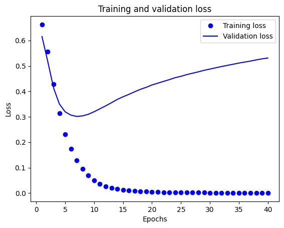
plt.title('Training and validation loss')
plt.xlabel('Epochs')
plt.ylabel('Loss')
plt.legend()
plt.show()
plt.clf()   # clear figure

plt.plot(epochs, acc, 'bo', label='Training acc')
plt.plot(epochs, val_acc, 'b', label='Validation acc')
plt.title('Training and validation accuracy')
plt.xlabel('Epochs')
plt.ylabel('Accuracy')
plt.legend()

plt.show()
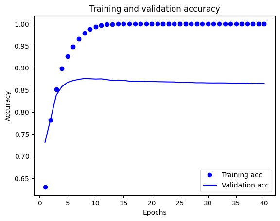
در این نمودار، نقاط نشان دهنده فقدان تمرین و دقت و خطوط ثابت، از دست دادن اعتبار و دقت هستند.
توجه داشته باشید که از دست دادن آموزش با هر دوره و آموزش دقت با هر دوره کاهش می یابد. هنگام استفاده از بهینهسازی نزولی گرادیان، این مورد انتظار میرود - باید مقدار مورد نظر را در هر تکرار به حداقل برساند.
این مورد در مورد از دست دادن اعتبار و دقت صدق نمی کند - به نظر می رسد آنها پس از حدود بیست دوره به اوج خود می رسند. این مثالی از برازش بیش از حد است: این مدل در دادههای آموزشی بهتر از دادههایی که قبلاً ندیده بود، عمل میکند. پس از این مرحله، مدل بیش از حد بهینه سازی و یاد می گیرد بازنمایی خاص به داده های آموزشی که به داده ها از آزمون تعمیم دهیم.
برای این مورد خاص، ما میتوانیم با توقف تمرین پس از بیست یا چند دوره، از افزایش بیش از حد آن جلوگیری کنیم. بعداً خواهید دید که چگونه می توان این کار را به طور خودکار با یک تماس برگشتی انجام داد.
# MIT License
#
# Copyright (c) 2017 François Chollet
#
# Permission is hereby granted, free of charge, to any person obtaining a
# copy of this software and associated documentation files (the "Software"),
# to deal in the Software without restriction, including without limitation
# the rights to use, copy, modify, merge, publish, distribute, sublicense,
# and/or sell copies of the Software, and to permit persons to whom the
# Software is furnished to do so, subject to the following conditions:
#
# The above copyright notice and this permission notice shall be included in
# all copies or substantial portions of the Software.
#
# THE SOFTWARE IS PROVIDED "AS IS", WITHOUT WARRANTY OF ANY KIND, EXPRESS OR
# IMPLIED, INCLUDING BUT NOT LIMITED TO THE WARRANTIES OF MERCHANTABILITY,
# FITNESS FOR A PARTICULAR PURPOSE AND NONINFRINGEMENT. IN NO EVENT SHALL
# THE AUTHORS OR COPYRIGHT HOLDERS BE LIABLE FOR ANY CLAIM, DAMAGES OR OTHER
# LIABILITY, WHETHER IN AN ACTION OF CONTRACT, TORT OR OTHERWISE, ARISING
# FROM, OUT OF OR IN CONNECTION WITH THE SOFTWARE OR THE USE OR OTHER
# DEALINGS IN THE SOFTWARE.