
| | |  GitHub'da görüntüle GitHub'da görüntüle | |
Güvenlik açısından kritik olan (örneğin, tıbbi karar verme ve otonom sürüş) veya verilerin doğası gereği gürültülü olduğu (örneğin, doğal dil anlama) AI uygulamalarında, derin bir sınıflandırıcının belirsizliğini güvenilir bir şekilde ölçmesi önemlidir. Derin sınıflandırıcı, kendi sınırlamalarının ve kontrolü ne zaman insan uzmanlara devretmesi gerektiğinin farkında olmalıdır. Bu öğretici, Spectral-normalized Neural Gaussian Process ( SNGP ) adlı bir teknik kullanarak, derin bir sınıflandırıcının belirsizliği niceleme yeteneğinin nasıl geliştirileceğini gösterir.
SNGP'nin temel fikri, ağa basit değişiklikler uygulayarak derin bir sınıflandırıcının mesafe farkındalığını geliştirmektir. Bir modelin mesafe farkındalığı , tahmine dayalı olasılığının test örneği ile eğitim verileri arasındaki mesafeyi nasıl yansıttığının bir ölçüsüdür. Bu, altın standart olasılıklı modeller için yaygın olan arzu edilen bir özelliktir (örneğin, RBF çekirdekli Gauss süreci ), ancak derin sinir ağlarına sahip modellerde eksiktir. SNGP, tahmin doğruluğunu korurken bu Gauss süreci davranışını derin bir sınıflandırıcıya yerleştirmek için basit bir yol sağlar.
Bu öğretici, iki ay veri setinde derin artık ağ (ResNet) tabanlı bir SNGP modeli uygular ve belirsizlik yüzeyini diğer iki popüler belirsizlik yaklaşımınınkiyle karşılaştırır - Monte Carlo bırakma ve Derin topluluk ).
Bu öğretici, bir oyuncak 2B veri kümesindeki SNGP modelini gösterir. BERT-tabanını kullanarak gerçek dünyadaki bir doğal dil anlama görevine SNGP uygulama örneği için lütfen SNGP-BERT öğreticisine bakın. SNGP modelinin (ve diğer birçok belirsizlik yönteminin) çok çeşitli kıyaslama veri kümelerinde ( örn .
SNGP hakkında
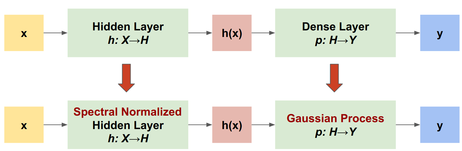
Spektral normalleştirilmiş Nöral Gauss Süreci (SNGP), benzer bir doğruluk ve gecikme seviyesini korurken derin bir sınıflandırıcının belirsizlik kalitesini iyileştirmek için basit bir yaklaşımdır. Derin bir artık ağ verildiğinde, SNGP modelde iki basit değişiklik yapar:
- Gizli kalıntı katmanlara spektral normalleştirme uygular.
- Yoğun çıktı katmanını bir Gauss işlem katmanıyla değiştirir.
Diğer belirsizlik yaklaşımlarıyla (örneğin, Monte Carlo bırakma veya Derin topluluk) karşılaştırıldığında, SNGP'nin çeşitli avantajları vardır:
- Çok çeşitli son teknoloji kalıntı tabanlı mimariler için çalışır (örn. (Wide) ResNet, DenseNet, BERT, vb.).
- Tek modelli bir yöntemdir (yani, topluluk ortalamasına dayanmaz). Bu nedenle SNGP, tek bir deterministik ağ ile benzer bir gecikme düzeyine sahiptir ve ImageNet ve Jigsaw Toxic Comments sınıflandırması gibi büyük veri kümelerine kolayca ölçeklenebilir.
- Mesafe farkındalığı özelliği nedeniyle güçlü alan dışı algılama performansına sahiptir.
Bu yöntemin dezavantajları şunlardır:
Bir SNGP'nin tahmine dayalı belirsizliği, Laplace yaklaşımı kullanılarak hesaplanır. Bu nedenle teorik olarak, SNGP'nin arka belirsizliği, kesin bir Gauss sürecininkinden farklıdır.
SNGP eğitimi, yeni bir çağın başlangıcında bir kovaryans sıfırlama adımına ihtiyaç duyar. Bu, bir eğitim hattına çok az miktarda ekstra karmaşıklık ekleyebilir. Bu öğretici, Keras geri aramalarını kullanarak bunu uygulamanın basit bir yolunu gösterir.
Kurmak
pip install --use-deprecated=legacy-resolver tf-models-official
# refresh pkg_resources so it takes the changes into account.
import pkg_resources
import importlib
importlib.reload(pkg_resources)
<module 'pkg_resources' from '/tmpfs/src/tf_docs_env/lib/python3.7/site-packages/pkg_resources/__init__.py'>
import matplotlib.pyplot as plt
import matplotlib.colors as colors

import sklearn.datasets

import numpy as np
import tensorflow as tf

import official.nlp.modeling.layers as nlp_layers
Görselleştirme makrolarını tanımlayın
plt.rcParams['figure.dpi'] = 140

DEFAULT_X_RANGE = (-3.5, 3.5)
DEFAULT_Y_RANGE = (-2.5, 2.5)
DEFAULT_CMAP = colors.ListedColormap(["#377eb8", "#ff7f00"])
DEFAULT_NORM = colors.Normalize(vmin=0, vmax=1,)
DEFAULT_N_GRID = 100
iki ay veri seti
İki ay veri setinden eğitim ve değerlendirme veri setlerini oluşturun.
def make_training_data(sample_size=500):
  """Create two moon training dataset."""
  train_examples, train_labels = sklearn.datasets.make_moons(
      n_samples=2 * sample_size, noise=0.1)

  # Adjust data position slightly.
  train_examples[train_labels == 0] += [-0.1, 0.2]
  train_examples[train_labels == 1] += [0.1, -0.2]

  return train_examples, train_labels
Modelin tahmine dayalı davranışını tüm 2B giriş alanı üzerinden değerlendirin.
def make_testing_data(x_range=DEFAULT_X_RANGE, y_range=DEFAULT_Y_RANGE, n_grid=DEFAULT_N_GRID):
  """Create a mesh grid in 2D space."""
  # testing data (mesh grid over data space)
  x = np.linspace(x_range[0], x_range[1], n_grid)
  y = np.linspace(y_range[0], y_range[1], n_grid)
  xv, yv = np.meshgrid(x, y)
  return np.stack([xv.flatten(), yv.flatten()], axis=-1)
Model belirsizliğini değerlendirmek için üçüncü sınıfa ait bir etki alanı dışı (OOD) veri kümesi ekleyin. Model, eğitim sırasında bu OOD örneklerini asla görmez.
def make_ood_data(sample_size=500, means=(2.5, -1.75), vars=(0.01, 0.01)):
  return np.random.multivariate_normal(
      means, cov=np.diag(vars), size=sample_size)
# Load the train, test and OOD datasets.
train_examples, train_labels = make_training_data(
    sample_size=500)
test_examples = make_testing_data()
ood_examples = make_ood_data(sample_size=500)

# Visualize
pos_examples = train_examples[train_labels == 0]
neg_examples = train_examples[train_labels == 1]

plt.figure(figsize=(7, 5.5))

plt.scatter(pos_examples[:, 0], pos_examples[:, 1], c="#377eb8", alpha=0.5)
plt.scatter(neg_examples[:, 0], neg_examples[:, 1], c="#ff7f00", alpha=0.5)
plt.scatter(ood_examples[:, 0], ood_examples[:, 1], c="red", alpha=0.1)

plt.legend(["Postive", "Negative", "Out-of-Domain"])

plt.ylim(DEFAULT_Y_RANGE)
plt.xlim(DEFAULT_X_RANGE)

plt.show()

Burada mavi ve turuncu, pozitif ve negatif sınıfları temsil eder ve kırmızı, OOD verilerini temsil eder. Belirsizliği iyi ölçen bir modelin eğitim verilerine yakın olduğunda (yani, \(p(x_{test})\) 0 veya 1'e yakın olduğunda) kendinden emin olması ve eğitim verisi bölgelerinden uzaktayken (yani, \(p(x_{test})\) 0,5'e yakın olduğunda) belirsiz olması beklenir. ).
deterministik model
modeli tanımla
(Temel) deterministik modelden başlayın: bırakma düzenlemeli çok katmanlı bir artık ağ (ResNet).
class DeepResNet(tf.keras.Model):
  """Defines a multi-layer residual network."""
  def __init__(self, num_classes, num_layers=3, num_hidden=128,
               dropout_rate=0.1, **classifier_kwargs):
    super().__init__()
    # Defines class meta data.
    self.num_hidden = num_hidden
    self.num_layers = num_layers
    self.dropout_rate = dropout_rate
    self.classifier_kwargs = classifier_kwargs

    # Defines the hidden layers.
    self.input_layer = tf.keras.layers.Dense(self.num_hidden, trainable=False)
    self.dense_layers = [self.make_dense_layer() for _ in range(num_layers)]

    # Defines the output layer.
    self.classifier = self.make_output_layer(num_classes)

  def call(self, inputs):
    # Projects the 2d input data to high dimension.
    hidden = self.input_layer(inputs)

    # Computes the resnet hidden representations.
    for i in range(self.num_layers):
      resid = self.dense_layers[i](hidden)
      resid = tf.keras.layers.Dropout(self.dropout_rate)(resid)
      hidden += resid

    return self.classifier(hidden)

  def make_dense_layer(self):
    """Uses the Dense layer as the hidden layer."""
    return tf.keras.layers.Dense(self.num_hidden, activation="relu")

  def make_output_layer(self, num_classes):
    """Uses the Dense layer as the output layer."""
    return tf.keras.layers.Dense(
        num_classes, **self.classifier_kwargs)
Bu öğretici, 128 gizli birim içeren 6 katmanlı bir ResNet kullanır.
resnet_config = dict(num_classes=2, num_layers=6, num_hidden=128)
resnet_model = DeepResNet(**resnet_config)
resnet_model.build((None, 2))
resnet_model.summary()
Model: "deep_res_net"
_________________________________________________________________
 Layer (type)                Output Shape              Param #
=================================================================
 dense (Dense)               multiple                  384

 dense_1 (Dense)             multiple                  16512

 dense_2 (Dense)             multiple                  16512

 dense_3 (Dense)             multiple                  16512

 dense_4 (Dense)             multiple                  16512

 dense_5 (Dense)             multiple                  16512

 dense_6 (Dense)             multiple                  16512

 dense_7 (Dense)             multiple                  258

=================================================================
Total params: 99,714
Trainable params: 99,330
Non-trainable params: 384
_________________________________________________________________
tren modeli
Kayıp işlevi ve Adam optimize edici olarak SparseCategoricalCrossentropy kullanmak için eğitim parametrelerini yapılandırın.
loss = tf.keras.losses.SparseCategoricalCrossentropy(from_logits=True)
metrics = tf.keras.metrics.SparseCategoricalAccuracy(),
optimizer = tf.keras.optimizers.Adam(learning_rate=1e-4)

train_config = dict(loss=loss, metrics=metrics, optimizer=optimizer)
Modeli, parti boyutu 128 ile 100 dönem için eğitin.
fit_config = dict(batch_size=128, epochs=100)
resnet_model.compile(**train_config)
resnet_model.fit(train_examples, train_labels, **fit_config)
Epoch 1/100
8/8 [==============================] - 1s 4ms/step - loss: 1.1251 - sparse_categorical_accuracy: 0.5050
Epoch 2/100
8/8 [==============================] - 0s 3ms/step - loss: 0.5538 - sparse_categorical_accuracy: 0.6920
Epoch 3/100
8/8 [==============================] - 0s 3ms/step - loss: 0.2881 - sparse_categorical_accuracy: 0.9160
Epoch 4/100
8/8 [==============================] - 0s 3ms/step - loss: 0.1923 - sparse_categorical_accuracy: 0.9370
Epoch 5/100
8/8 [==============================] - 0s 3ms/step - loss: 0.1550 - sparse_categorical_accuracy: 0.9420
Epoch 6/100
8/8 [==============================] - 0s 3ms/step - loss: 0.1403 - sparse_categorical_accuracy: 0.9450
Epoch 7/100
8/8 [==============================] - 0s 3ms/step - loss: 0.1269 - sparse_categorical_accuracy: 0.9430
Epoch 8/100
8/8 [==============================] - 0s 3ms/step - loss: 0.1208 - sparse_categorical_accuracy: 0.9460
Epoch 9/100
8/8 [==============================] - 0s 3ms/step - loss: 0.1158 - sparse_categorical_accuracy: 0.9510
Epoch 10/100
8/8 [==============================] - 0s 3ms/step - loss: 0.1103 - sparse_categorical_accuracy: 0.9490
Epoch 11/100
8/8 [==============================] - 0s 3ms/step - loss: 0.1051 - sparse_categorical_accuracy: 0.9510
Epoch 12/100
8/8 [==============================] - 0s 3ms/step - loss: 0.1053 - sparse_categorical_accuracy: 0.9510
Epoch 13/100
8/8 [==============================] - 0s 3ms/step - loss: 0.1013 - sparse_categorical_accuracy: 0.9450
Epoch 14/100
8/8 [==============================] - 0s 4ms/step - loss: 0.0967 - sparse_categorical_accuracy: 0.9500
Epoch 15/100
8/8 [==============================] - 0s 3ms/step - loss: 0.0991 - sparse_categorical_accuracy: 0.9530
Epoch 16/100
8/8 [==============================] - 0s 3ms/step - loss: 0.0984 - sparse_categorical_accuracy: 0.9500
Epoch 17/100
8/8 [==============================] - 0s 3ms/step - loss: 0.0982 - sparse_categorical_accuracy: 0.9480
Epoch 18/100
8/8 [==============================] - 0s 4ms/step - loss: 0.0918 - sparse_categorical_accuracy: 0.9510
Epoch 19/100
8/8 [==============================] - 0s 3ms/step - loss: 0.0903 - sparse_categorical_accuracy: 0.9500
Epoch 20/100
8/8 [==============================] - 0s 3ms/step - loss: 0.0883 - sparse_categorical_accuracy: 0.9510
Epoch 21/100
8/8 [==============================] - 0s 3ms/step - loss: 0.0870 - sparse_categorical_accuracy: 0.9530
Epoch 22/100
8/8 [==============================] - 0s 3ms/step - loss: 0.0884 - sparse_categorical_accuracy: 0.9560
Epoch 23/100
8/8 [==============================] - 0s 3ms/step - loss: 0.0850 - sparse_categorical_accuracy: 0.9540
Epoch 24/100
8/8 [==============================] - 0s 3ms/step - loss: 0.0808 - sparse_categorical_accuracy: 0.9580
Epoch 25/100
8/8 [==============================] - 0s 3ms/step - loss: 0.0773 - sparse_categorical_accuracy: 0.9560
Epoch 26/100
8/8 [==============================] - 0s 3ms/step - loss: 0.0801 - sparse_categorical_accuracy: 0.9590
Epoch 27/100
8/8 [==============================] - 0s 3ms/step - loss: 0.0779 - sparse_categorical_accuracy: 0.9580
Epoch 28/100
8/8 [==============================] - 0s 3ms/step - loss: 0.0807 - sparse_categorical_accuracy: 0.9580
Epoch 29/100
8/8 [==============================] - 0s 3ms/step - loss: 0.0820 - sparse_categorical_accuracy: 0.9570
Epoch 30/100
8/8 [==============================] - 0s 3ms/step - loss: 0.0730 - sparse_categorical_accuracy: 0.9600
Epoch 31/100
8/8 [==============================] - 0s 3ms/step - loss: 0.0782 - sparse_categorical_accuracy: 0.9590
Epoch 32/100
8/8 [==============================] - 0s 4ms/step - loss: 0.0704 - sparse_categorical_accuracy: 0.9600
Epoch 33/100
8/8 [==============================] - 0s 3ms/step - loss: 0.0709 - sparse_categorical_accuracy: 0.9610
Epoch 34/100
8/8 [==============================] - 0s 3ms/step - loss: 0.0758 - sparse_categorical_accuracy: 0.9580
Epoch 35/100
8/8 [==============================] - 0s 3ms/step - loss: 0.0702 - sparse_categorical_accuracy: 0.9610
Epoch 36/100
8/8 [==============================] - 0s 3ms/step - loss: 0.0688 - sparse_categorical_accuracy: 0.9600
Epoch 37/100
8/8 [==============================] - 0s 3ms/step - loss: 0.0675 - sparse_categorical_accuracy: 0.9630
Epoch 38/100
8/8 [==============================] - 0s 3ms/step - loss: 0.0636 - sparse_categorical_accuracy: 0.9690
Epoch 39/100
8/8 [==============================] - 0s 3ms/step - loss: 0.0677 - sparse_categorical_accuracy: 0.9610
Epoch 40/100
8/8 [==============================] - 0s 3ms/step - loss: 0.0702 - sparse_categorical_accuracy: 0.9650
Epoch 41/100
8/8 [==============================] - 0s 3ms/step - loss: 0.0614 - sparse_categorical_accuracy: 0.9690
Epoch 42/100
8/8 [==============================] - 0s 3ms/step - loss: 0.0663 - sparse_categorical_accuracy: 0.9680
Epoch 43/100
8/8 [==============================] - 0s 3ms/step - loss: 0.0626 - sparse_categorical_accuracy: 0.9740
Epoch 44/100
8/8 [==============================] - 0s 3ms/step - loss: 0.0590 - sparse_categorical_accuracy: 0.9760
Epoch 45/100
8/8 [==============================] - 0s 3ms/step - loss: 0.0573 - sparse_categorical_accuracy: 0.9780
Epoch 46/100
8/8 [==============================] - 0s 3ms/step - loss: 0.0568 - sparse_categorical_accuracy: 0.9770
Epoch 47/100
8/8 [==============================] - 0s 3ms/step - loss: 0.0595 - sparse_categorical_accuracy: 0.9780
Epoch 48/100
8/8 [==============================] - 0s 3ms/step - loss: 0.0482 - sparse_categorical_accuracy: 0.9840
Epoch 49/100
8/8 [==============================] - 0s 3ms/step - loss: 0.0515 - sparse_categorical_accuracy: 0.9820
Epoch 50/100
8/8 [==============================] - 0s 3ms/step - loss: 0.0525 - sparse_categorical_accuracy: 0.9830
Epoch 51/100
8/8 [==============================] - 0s 3ms/step - loss: 0.0507 - sparse_categorical_accuracy: 0.9790
Epoch 52/100
8/8 [==============================] - 0s 3ms/step - loss: 0.0433 - sparse_categorical_accuracy: 0.9850
Epoch 53/100
8/8 [==============================] - 0s 3ms/step - loss: 0.0511 - sparse_categorical_accuracy: 0.9820
Epoch 54/100
8/8 [==============================] - 0s 3ms/step - loss: 0.0501 - sparse_categorical_accuracy: 0.9820
Epoch 55/100
8/8 [==============================] - 0s 3ms/step - loss: 0.0440 - sparse_categorical_accuracy: 0.9890
Epoch 56/100
8/8 [==============================] - 0s 3ms/step - loss: 0.0438 - sparse_categorical_accuracy: 0.9850
Epoch 57/100
8/8 [==============================] - 0s 3ms/step - loss: 0.0438 - sparse_categorical_accuracy: 0.9880
Epoch 58/100
8/8 [==============================] - 0s 3ms/step - loss: 0.0416 - sparse_categorical_accuracy: 0.9860
Epoch 59/100
8/8 [==============================] - 0s 3ms/step - loss: 0.0479 - sparse_categorical_accuracy: 0.9860
Epoch 60/100
8/8 [==============================] - 0s 3ms/step - loss: 0.0434 - sparse_categorical_accuracy: 0.9860
Epoch 61/100
8/8 [==============================] - 0s 3ms/step - loss: 0.0414 - sparse_categorical_accuracy: 0.9880
Epoch 62/100
8/8 [==============================] - 0s 3ms/step - loss: 0.0402 - sparse_categorical_accuracy: 0.9870
Epoch 63/100
8/8 [==============================] - 0s 3ms/step - loss: 0.0376 - sparse_categorical_accuracy: 0.9890
Epoch 64/100
8/8 [==============================] - 0s 3ms/step - loss: 0.0337 - sparse_categorical_accuracy: 0.9900
Epoch 65/100
8/8 [==============================] - 0s 3ms/step - loss: 0.0309 - sparse_categorical_accuracy: 0.9910
Epoch 66/100
8/8 [==============================] - 0s 3ms/step - loss: 0.0336 - sparse_categorical_accuracy: 0.9910
Epoch 67/100
8/8 [==============================] - 0s 3ms/step - loss: 0.0389 - sparse_categorical_accuracy: 0.9870
Epoch 68/100
8/8 [==============================] - 0s 3ms/step - loss: 0.0333 - sparse_categorical_accuracy: 0.9920
Epoch 69/100
8/8 [==============================] - 0s 3ms/step - loss: 0.0331 - sparse_categorical_accuracy: 0.9890
Epoch 70/100
8/8 [==============================] - 0s 3ms/step - loss: 0.0346 - sparse_categorical_accuracy: 0.9900
Epoch 71/100
8/8 [==============================] - 0s 3ms/step - loss: 0.0367 - sparse_categorical_accuracy: 0.9880
Epoch 72/100
8/8 [==============================] - 0s 3ms/step - loss: 0.0283 - sparse_categorical_accuracy: 0.9920
Epoch 73/100
8/8 [==============================] - 0s 3ms/step - loss: 0.0315 - sparse_categorical_accuracy: 0.9930
Epoch 74/100
8/8 [==============================] - 0s 3ms/step - loss: 0.0271 - sparse_categorical_accuracy: 0.9900
Epoch 75/100
8/8 [==============================] - 0s 3ms/step - loss: 0.0257 - sparse_categorical_accuracy: 0.9920
Epoch 76/100
8/8 [==============================] - 0s 3ms/step - loss: 0.0289 - sparse_categorical_accuracy: 0.9900
Epoch 77/100
8/8 [==============================] - 0s 3ms/step - loss: 0.0264 - sparse_categorical_accuracy: 0.9900
Epoch 78/100
8/8 [==============================] - 0s 3ms/step - loss: 0.0272 - sparse_categorical_accuracy: 0.9910
Epoch 79/100
8/8 [==============================] - 0s 3ms/step - loss: 0.0336 - sparse_categorical_accuracy: 0.9880
Epoch 80/100
8/8 [==============================] - 0s 3ms/step - loss: 0.0249 - sparse_categorical_accuracy: 0.9900
Epoch 81/100
8/8 [==============================] - 0s 3ms/step - loss: 0.0216 - sparse_categorical_accuracy: 0.9930
Epoch 82/100
8/8 [==============================] - 0s 3ms/step - loss: 0.0279 - sparse_categorical_accuracy: 0.9890
Epoch 83/100
8/8 [==============================] - 0s 3ms/step - loss: 0.0261 - sparse_categorical_accuracy: 0.9920
Epoch 84/100
8/8 [==============================] - 0s 3ms/step - loss: 0.0235 - sparse_categorical_accuracy: 0.9920
Epoch 85/100
8/8 [==============================] - 0s 3ms/step - loss: 0.0236 - sparse_categorical_accuracy: 0.9930
Epoch 86/100
8/8 [==============================] - 0s 3ms/step - loss: 0.0219 - sparse_categorical_accuracy: 0.9920
Epoch 87/100
8/8 [==============================] - 0s 3ms/step - loss: 0.0196 - sparse_categorical_accuracy: 0.9920
Epoch 88/100
8/8 [==============================] - 0s 3ms/step - loss: 0.0215 - sparse_categorical_accuracy: 0.9900
Epoch 89/100
8/8 [==============================] - 0s 3ms/step - loss: 0.0223 - sparse_categorical_accuracy: 0.9900
Epoch 90/100
8/8 [==============================] - 0s 3ms/step - loss: 0.0200 - sparse_categorical_accuracy: 0.9950
Epoch 91/100
8/8 [==============================] - 0s 3ms/step - loss: 0.0250 - sparse_categorical_accuracy: 0.9900
Epoch 92/100
8/8 [==============================] - 0s 3ms/step - loss: 0.0160 - sparse_categorical_accuracy: 0.9940
Epoch 93/100
8/8 [==============================] - 0s 3ms/step - loss: 0.0203 - sparse_categorical_accuracy: 0.9930
Epoch 94/100
8/8 [==============================] - 0s 3ms/step - loss: 0.0203 - sparse_categorical_accuracy: 0.9930
Epoch 95/100
8/8 [==============================] - 0s 3ms/step - loss: 0.0172 - sparse_categorical_accuracy: 0.9960
Epoch 96/100
8/8 [==============================] - 0s 3ms/step - loss: 0.0209 - sparse_categorical_accuracy: 0.9940
Epoch 97/100
8/8 [==============================] - 0s 3ms/step - loss: 0.0179 - sparse_categorical_accuracy: 0.9920
Epoch 98/100
8/8 [==============================] - 0s 3ms/step - loss: 0.0195 - sparse_categorical_accuracy: 0.9940
Epoch 99/100
8/8 [==============================] - 0s 3ms/step - loss: 0.0165 - sparse_categorical_accuracy: 0.9930
Epoch 100/100
8/8 [==============================] - 0s 3ms/step - loss: 0.0170 - sparse_categorical_accuracy: 0.9950
<keras.callbacks.History at 0x7ff7ac5c8fd0>
Belirsizliği görselleştirin
def plot_uncertainty_surface(test_uncertainty, ax, cmap=None):
  """Visualizes the 2D uncertainty surface.

  For simplicity, assume these objects already exist in the memory:

    test_examples: Array of test examples, shape (num_test, 2).
    train_labels: Array of train labels, shape (num_train, ).
    train_examples: Array of train examples, shape (num_train, 2).

  Arguments:
    test_uncertainty: Array of uncertainty scores, shape (num_test,).
    ax: A matplotlib Axes object that specifies a matplotlib figure.
    cmap: A matplotlib colormap object specifying the palette of the
      predictive surface.

  Returns:
    pcm: A matplotlib PathCollection object that contains the palette
      information of the uncertainty plot.
  """
  # Normalize uncertainty for better visualization.
  test_uncertainty = test_uncertainty / np.max(test_uncertainty)

  # Set view limits.
  ax.set_ylim(DEFAULT_Y_RANGE)
  ax.set_xlim(DEFAULT_X_RANGE)

  # Plot normalized uncertainty surface.
  pcm = ax.imshow(
      np.reshape(test_uncertainty, [DEFAULT_N_GRID, DEFAULT_N_GRID]),
      cmap=cmap,
      origin="lower",
      extent=DEFAULT_X_RANGE + DEFAULT_Y_RANGE,
      vmin=DEFAULT_NORM.vmin,
      vmax=DEFAULT_NORM.vmax,
      interpolation='bicubic',
      aspect='auto')

  # Plot training data.
  ax.scatter(train_examples[:, 0], train_examples[:, 1],
             c=train_labels, cmap=DEFAULT_CMAP, alpha=0.5)
  ax.scatter(ood_examples[:, 0], ood_examples[:, 1], c="red", alpha=0.1)

  return pcm
Şimdi deterministik modelin tahminlerini görselleştirin. İlk önce sınıf olasılığını çizin:
\[p(x) = softmax(logit(x))\]
resnet_logits = resnet_model(test_examples)
resnet_probs = tf.nn.softmax(resnet_logits, axis=-1)[:, 0]  # Take the probability for class 0.
_, ax = plt.subplots(figsize=(7, 5.5))

pcm = plot_uncertainty_surface(resnet_probs, ax=ax)

plt.colorbar(pcm, ax=ax)
plt.title("Class Probability, Deterministic Model")

plt.show()

Bu grafikte, sarı ve mor, iki sınıf için tahmin olasılıklarıdır. Deterministik model, doğrusal olmayan bir karar sınırı ile bilinen iki sınıfı (mavi ve turuncu) sınıflandırmada iyi bir iş çıkardı. Ancak, mesafe farkında değildir ve hiç görülmemiş kırmızı alan dışı (OOD) örneklerini güvenle turuncu sınıf olarak sınıflandırır.
Tahmine dayalı varyansı hesaplayarak model belirsizliğini görselleştirin:
\[var(x) = p(x) * (1 - p(x))\]
resnet_uncertainty = resnet_probs * (1 - resnet_probs)
_, ax = plt.subplots(figsize=(7, 5.5))

pcm = plot_uncertainty_surface(resnet_uncertainty, ax=ax)

plt.colorbar(pcm, ax=ax)
plt.title("Predictive Uncertainty, Deterministic Model")

plt.show()

Bu çizimde sarı, yüksek belirsizliği, mor ise düşük belirsizliği gösterir. Deterministik ResNet'in belirsizliği, yalnızca test örneklerinin karar sınırından uzaklığına bağlıdır. Bu, modelin eğitim alanının dışındayken aşırı özgüvenli olmasına yol açar. Sonraki bölüm, SNGP'nin bu veri kümesinde nasıl farklı davrandığını gösterir.
SNGP modeli
SNGP modelini tanımlayın
Şimdi SNGP modelini uygulayalım. SNGP bileşenlerinin her ikisi de, SpectralNormalization ve RandomFeatureGaussianProcess , tensorflow_model'in yerleşik katmanlarında mevcuttur.
Bu iki bileşene daha ayrıntılı olarak bakalım. (Tam modelin nasıl uygulandığını görmek için SNGP modeli bölümüne de atlayabilirsiniz.)
Spektral Normalizasyon sarmalayıcısı
SpectralNormalization , bir Keras katman sarıcısıdır. Mevcut bir Yoğun katmana şu şekilde uygulanabilir:
dense = tf.keras.layers.Dense(units=10)
dense = nlp_layers.SpectralNormalization(dense, norm_multiplier=0.9)
Spektral normalleştirme, spektral normunu (yani, \(W\)en büyük özdeğerini) hedef değer norm_multiplier doğru kademeli olarak yönlendirerek gizli ağırlığı \(W\) düzenler.
Gauss Süreci (GP) katmanı
RandomFeatureGaussianProcess , derin bir sinir ağı ile uçtan uca eğitilebilir bir Gauss süreç modeline rastgele özellik tabanlı bir yaklaşım uygular. Kaputun altında, Gauss işlem katmanı iki katmanlı bir ağ uygular:
\[logits(x) = \Phi(x) \beta, \quad \Phi(x)=\sqrt{\frac{2}{M} } * cos(Wx + b)\]
Burada \(x\) girdidir ve \(W\) tutucu9 ve \(b\) sırasıyla Gauss ve düzgün dağılımlardan rastgele başlatılan dondurulmuş ağırlıklardır. (Bu nedenle \(\Phi(x)\) "rastgele özellikler" olarak adlandırılır.) \(\beta\) , Dense katmanına benzer öğrenilebilir çekirdek ağırlığıdır.
batch_size = 32
input_dim = 1024
num_classes = 10
gp_layer = nlp_layers.RandomFeatureGaussianProcess(units=num_classes,
                                               num_inducing=1024,
                                               normalize_input=False,
                                               scale_random_features=True,
                                               gp_cov_momentum=-1)
GP katmanlarının ana parametreleri şunlardır:
-
units: Çıkış logitlerinin boyutu. -
num_inducing: \(M\) gizli ağırlığının \(W\)boyutu. 1024'e varsayılan. -
normalize_input: \(x\)girişine katman normalleştirme uygulanıp uygulanmayacağı. -
scale_random_features: \(\sqrt{2/M}\) ölçeğinin gizli çıktıya uygulanıp uygulanmayacağını belirtir.
-
gp_cov_momentum, model kovaryansının nasıl hesaplandığını kontrol eder. Pozitif bir değere ayarlanırsa (örneğin, 0,999), kovaryans matrisi, momentuma dayalı hareketli ortalama güncellemesi kullanılarak hesaplanır (parti normalizasyonuna benzer). -1'e ayarlanırsa kovaryans matrisi momentum olmadan güncellenir.
Shape (batch_size, input_dim) ile bir toplu girdi verildiğinde, GP katmanı tahmin için bir logits tensörünü (shape (batch_size, (batch_size, num_classes) )) ve ayrıca arka kovaryans matrisi olan covmat tensörünü (shape (batch_size, batch_size) ) döndürür. toplu logit'ler.
embedding = tf.random.normal(shape=(batch_size, input_dim))

logits, covmat = gp_layer(embedding)
Teorik olarak, algoritmayı farklı sınıflar için farklı varyans değerlerini hesaplayacak şekilde genişletmek mümkündür ( orijinal SNGP belgesinde tanıtıldığı gibi). Ancak, bunun geniş çıktı alanları (örneğin, ImageNet veya dil modelleme) ile ilgili sorunlara ölçeklenmesi zordur.
Tam SNGP modeli
DeepResNet temel sınıfı göz önüne alındığında, SNGP modeli, artık ağın gizli ve çıkış katmanlarını değiştirerek kolayca uygulanabilir. model.fit() API ile uyumluluk için, modelin call() yöntemini de değiştirin, böylece eğitim sırasında yalnızca logits çıktısı verir.
class DeepResNetSNGP(DeepResNet):
  def __init__(self, spec_norm_bound=0.9, **kwargs):
    self.spec_norm_bound = spec_norm_bound
    super().__init__(**kwargs)

  def make_dense_layer(self):
    """Applies spectral normalization to the hidden layer."""
    dense_layer = super().make_dense_layer()
    return nlp_layers.SpectralNormalization(
        dense_layer, norm_multiplier=self.spec_norm_bound)

  def make_output_layer(self, num_classes):
    """Uses Gaussian process as the output layer."""
    return nlp_layers.RandomFeatureGaussianProcess(
        num_classes,
        gp_cov_momentum=-1,
        **self.classifier_kwargs)

  def call(self, inputs, training=False, return_covmat=False):
    # Gets logits and covariance matrix from GP layer.
    logits, covmat = super().call(inputs)

    # Returns only logits during training.
    if not training and return_covmat:
      return logits, covmat

    return logits
Deterministik modelle aynı mimariyi kullanın.
resnet_config
{'num_classes': 2, 'num_layers': 6, 'num_hidden': 128}
sngp_model = DeepResNetSNGP(**resnet_config)
sngp_model.build((None, 2))
sngp_model.summary()
Model: "deep_res_net_sngp"
_________________________________________________________________
 Layer (type)                Output Shape              Param #
=================================================================
 dense_9 (Dense)             multiple                  384

 spectral_normalization_1 (S  multiple                 16768
 pectralNormalization)

 spectral_normalization_2 (S  multiple                 16768
 pectralNormalization)

 spectral_normalization_3 (S  multiple                 16768
 pectralNormalization)

 spectral_normalization_4 (S  multiple                 16768
 pectralNormalization)

 spectral_normalization_5 (S  multiple                 16768
 pectralNormalization)

 spectral_normalization_6 (S  multiple                 16768
 pectralNormalization)

 random_feature_gaussian_pro  multiple                 1182722
 cess (RandomFeatureGaussian
 Process)

=================================================================
Total params: 1,283,714
Trainable params: 101,120
Non-trainable params: 1,182,594
_________________________________________________________________
Yeni bir çağın başlangıcında kovaryans matrisini sıfırlamak için bir Keras geri araması uygulayın.
class ResetCovarianceCallback(tf.keras.callbacks.Callback):

  def on_epoch_begin(self, epoch, logs=None):
    """Resets covariance matrix at the begining of the epoch."""
    if epoch > 0:
      self.model.classifier.reset_covariance_matrix()
Bu geri DeepResNetSNGP model sınıfına ekleyin.
class DeepResNetSNGPWithCovReset(DeepResNetSNGP):
  def fit(self, *args, **kwargs):
    """Adds ResetCovarianceCallback to model callbacks."""
    kwargs["callbacks"] = list(kwargs.get("callbacks", []))
    kwargs["callbacks"].append(ResetCovarianceCallback())

    return super().fit(*args, **kwargs)
tren modeli
Modeli eğitmek için tf.keras.model.fit kullanın.
sngp_model = DeepResNetSNGPWithCovReset(**resnet_config)
sngp_model.compile(**train_config)
sngp_model.fit(train_examples, train_labels, **fit_config)
Epoch 1/100
8/8 [==============================] - 2s 5ms/step - loss: 0.6223 - sparse_categorical_accuracy: 0.9570
Epoch 2/100
8/8 [==============================] - 0s 4ms/step - loss: 0.5310 - sparse_categorical_accuracy: 0.9980
Epoch 3/100
8/8 [==============================] - 0s 4ms/step - loss: 0.4766 - sparse_categorical_accuracy: 0.9990
Epoch 4/100
8/8 [==============================] - 0s 5ms/step - loss: 0.4346 - sparse_categorical_accuracy: 0.9980
Epoch 5/100
8/8 [==============================] - 0s 5ms/step - loss: 0.4015 - sparse_categorical_accuracy: 0.9980
Epoch 6/100
8/8 [==============================] - 0s 5ms/step - loss: 0.3757 - sparse_categorical_accuracy: 0.9990
Epoch 7/100
8/8 [==============================] - 0s 4ms/step - loss: 0.3525 - sparse_categorical_accuracy: 0.9990
Epoch 8/100
8/8 [==============================] - 0s 4ms/step - loss: 0.3305 - sparse_categorical_accuracy: 0.9990
Epoch 9/100
8/8 [==============================] - 0s 5ms/step - loss: 0.3144 - sparse_categorical_accuracy: 0.9980
Epoch 10/100
8/8 [==============================] - 0s 5ms/step - loss: 0.2975 - sparse_categorical_accuracy: 0.9990
Epoch 11/100
8/8 [==============================] - 0s 4ms/step - loss: 0.2832 - sparse_categorical_accuracy: 0.9990
Epoch 12/100
8/8 [==============================] - 0s 5ms/step - loss: 0.2707 - sparse_categorical_accuracy: 0.9990
Epoch 13/100
8/8 [==============================] - 0s 4ms/step - loss: 0.2568 - sparse_categorical_accuracy: 0.9990
Epoch 14/100
8/8 [==============================] - 0s 4ms/step - loss: 0.2470 - sparse_categorical_accuracy: 0.9970
Epoch 15/100
8/8 [==============================] - 0s 4ms/step - loss: 0.2361 - sparse_categorical_accuracy: 0.9990
Epoch 16/100
8/8 [==============================] - 0s 5ms/step - loss: 0.2271 - sparse_categorical_accuracy: 0.9990
Epoch 17/100
8/8 [==============================] - 0s 5ms/step - loss: 0.2182 - sparse_categorical_accuracy: 0.9990
Epoch 18/100
8/8 [==============================] - 0s 4ms/step - loss: 0.2097 - sparse_categorical_accuracy: 0.9990
Epoch 19/100
8/8 [==============================] - 0s 4ms/step - loss: 0.2018 - sparse_categorical_accuracy: 0.9990
Epoch 20/100
8/8 [==============================] - 0s 4ms/step - loss: 0.1940 - sparse_categorical_accuracy: 0.9980
Epoch 21/100
8/8 [==============================] - 0s 4ms/step - loss: 0.1892 - sparse_categorical_accuracy: 0.9990
Epoch 22/100
8/8 [==============================] - 0s 4ms/step - loss: 0.1821 - sparse_categorical_accuracy: 0.9980
Epoch 23/100
8/8 [==============================] - 0s 4ms/step - loss: 0.1768 - sparse_categorical_accuracy: 0.9990
Epoch 24/100
8/8 [==============================] - 0s 4ms/step - loss: 0.1702 - sparse_categorical_accuracy: 0.9980
Epoch 25/100
8/8 [==============================] - 0s 4ms/step - loss: 0.1664 - sparse_categorical_accuracy: 0.9990
Epoch 26/100
8/8 [==============================] - 0s 4ms/step - loss: 0.1604 - sparse_categorical_accuracy: 0.9990
Epoch 27/100
8/8 [==============================] - 0s 4ms/step - loss: 0.1565 - sparse_categorical_accuracy: 0.9990
Epoch 28/100
8/8 [==============================] - 0s 4ms/step - loss: 0.1517 - sparse_categorical_accuracy: 0.9990
Epoch 29/100
8/8 [==============================] - 0s 4ms/step - loss: 0.1469 - sparse_categorical_accuracy: 0.9990
Epoch 30/100
8/8 [==============================] - 0s 4ms/step - loss: 0.1431 - sparse_categorical_accuracy: 0.9980
Epoch 31/100
8/8 [==============================] - 0s 4ms/step - loss: 0.1385 - sparse_categorical_accuracy: 0.9980
Epoch 32/100
8/8 [==============================] - 0s 4ms/step - loss: 0.1351 - sparse_categorical_accuracy: 0.9990
Epoch 33/100
8/8 [==============================] - 0s 5ms/step - loss: 0.1312 - sparse_categorical_accuracy: 0.9980
Epoch 34/100
8/8 [==============================] - 0s 4ms/step - loss: 0.1289 - sparse_categorical_accuracy: 0.9990
Epoch 35/100
8/8 [==============================] - 0s 4ms/step - loss: 0.1254 - sparse_categorical_accuracy: 0.9980
Epoch 36/100
8/8 [==============================] - 0s 4ms/step - loss: 0.1223 - sparse_categorical_accuracy: 0.9980
Epoch 37/100
8/8 [==============================] - 0s 4ms/step - loss: 0.1180 - sparse_categorical_accuracy: 0.9990
Epoch 38/100
8/8 [==============================] - 0s 4ms/step - loss: 0.1167 - sparse_categorical_accuracy: 0.9990
Epoch 39/100
8/8 [==============================] - 0s 4ms/step - loss: 0.1132 - sparse_categorical_accuracy: 0.9980
Epoch 40/100
8/8 [==============================] - 0s 4ms/step - loss: 0.1110 - sparse_categorical_accuracy: 0.9990
Epoch 41/100
8/8 [==============================] - 0s 4ms/step - loss: 0.1075 - sparse_categorical_accuracy: 0.9990
Epoch 42/100
8/8 [==============================] - 0s 4ms/step - loss: 0.1067 - sparse_categorical_accuracy: 0.9990
Epoch 43/100
8/8 [==============================] - 0s 4ms/step - loss: 0.1034 - sparse_categorical_accuracy: 0.9990
Epoch 44/100
8/8 [==============================] - 0s 4ms/step - loss: 0.1006 - sparse_categorical_accuracy: 0.9990
Epoch 45/100
8/8 [==============================] - 0s 5ms/step - loss: 0.0991 - sparse_categorical_accuracy: 0.9990
Epoch 46/100
8/8 [==============================] - 0s 5ms/step - loss: 0.0963 - sparse_categorical_accuracy: 0.9990
Epoch 47/100
8/8 [==============================] - 0s 5ms/step - loss: 0.0943 - sparse_categorical_accuracy: 0.9980
Epoch 48/100
8/8 [==============================] - 0s 5ms/step - loss: 0.0925 - sparse_categorical_accuracy: 0.9990
Epoch 49/100
8/8 [==============================] - 0s 4ms/step - loss: 0.0905 - sparse_categorical_accuracy: 0.9990
Epoch 50/100
8/8 [==============================] - 0s 5ms/step - loss: 0.0889 - sparse_categorical_accuracy: 0.9990
Epoch 51/100
8/8 [==============================] - 0s 5ms/step - loss: 0.0863 - sparse_categorical_accuracy: 0.9980
Epoch 52/100
8/8 [==============================] - 0s 5ms/step - loss: 0.0847 - sparse_categorical_accuracy: 0.9990
Epoch 53/100
8/8 [==============================] - 0s 5ms/step - loss: 0.0831 - sparse_categorical_accuracy: 0.9980
Epoch 54/100
8/8 [==============================] - 0s 5ms/step - loss: 0.0818 - sparse_categorical_accuracy: 0.9990
Epoch 55/100
8/8 [==============================] - 0s 5ms/step - loss: 0.0799 - sparse_categorical_accuracy: 0.9990
Epoch 56/100
8/8 [==============================] - 0s 4ms/step - loss: 0.0780 - sparse_categorical_accuracy: 0.9990
Epoch 57/100
8/8 [==============================] - 0s 5ms/step - loss: 0.0768 - sparse_categorical_accuracy: 0.9990
Epoch 58/100
8/8 [==============================] - 0s 4ms/step - loss: 0.0751 - sparse_categorical_accuracy: 0.9990
Epoch 59/100
8/8 [==============================] - 0s 4ms/step - loss: 0.0748 - sparse_categorical_accuracy: 0.9990
Epoch 60/100
8/8 [==============================] - 0s 4ms/step - loss: 0.0723 - sparse_categorical_accuracy: 0.9990
Epoch 61/100
8/8 [==============================] - 0s 4ms/step - loss: 0.0712 - sparse_categorical_accuracy: 0.9990
Epoch 62/100
8/8 [==============================] - 0s 4ms/step - loss: 0.0701 - sparse_categorical_accuracy: 0.9990
Epoch 63/100
8/8 [==============================] - 0s 4ms/step - loss: 0.0701 - sparse_categorical_accuracy: 0.9990
Epoch 64/100
8/8 [==============================] - 0s 4ms/step - loss: 0.0683 - sparse_categorical_accuracy: 0.9990
Epoch 65/100
8/8 [==============================] - 0s 5ms/step - loss: 0.0665 - sparse_categorical_accuracy: 0.9990
Epoch 66/100
8/8 [==============================] - 0s 5ms/step - loss: 0.0661 - sparse_categorical_accuracy: 0.9990
Epoch 67/100
8/8 [==============================] - 0s 5ms/step - loss: 0.0636 - sparse_categorical_accuracy: 0.9990
Epoch 68/100
8/8 [==============================] - 0s 4ms/step - loss: 0.0631 - sparse_categorical_accuracy: 0.9990
Epoch 69/100
8/8 [==============================] - 0s 4ms/step - loss: 0.0620 - sparse_categorical_accuracy: 0.9990
Epoch 70/100
8/8 [==============================] - 0s 5ms/step - loss: 0.0606 - sparse_categorical_accuracy: 0.9990
Epoch 71/100
8/8 [==============================] - 0s 4ms/step - loss: 0.0601 - sparse_categorical_accuracy: 0.9980
Epoch 72/100
8/8 [==============================] - 0s 4ms/step - loss: 0.0590 - sparse_categorical_accuracy: 0.9990
Epoch 73/100
8/8 [==============================] - 0s 4ms/step - loss: 0.0586 - sparse_categorical_accuracy: 0.9990
Epoch 74/100
8/8 [==============================] - 0s 4ms/step - loss: 0.0574 - sparse_categorical_accuracy: 0.9990
Epoch 75/100
8/8 [==============================] - 0s 4ms/step - loss: 0.0565 - sparse_categorical_accuracy: 1.0000
Epoch 76/100
8/8 [==============================] - 0s 4ms/step - loss: 0.0559 - sparse_categorical_accuracy: 0.9990
Epoch 77/100
8/8 [==============================] - 0s 4ms/step - loss: 0.0549 - sparse_categorical_accuracy: 0.9990
Epoch 78/100
8/8 [==============================] - 0s 5ms/step - loss: 0.0534 - sparse_categorical_accuracy: 1.0000
Epoch 79/100
8/8 [==============================] - 0s 5ms/step - loss: 0.0532 - sparse_categorical_accuracy: 0.9990
Epoch 80/100
8/8 [==============================] - 0s 4ms/step - loss: 0.0519 - sparse_categorical_accuracy: 1.0000
Epoch 81/100
8/8 [==============================] - 0s 4ms/step - loss: 0.0511 - sparse_categorical_accuracy: 1.0000
Epoch 82/100
8/8 [==============================] - 0s 4ms/step - loss: 0.0508 - sparse_categorical_accuracy: 0.9990
Epoch 83/100
8/8 [==============================] - 0s 4ms/step - loss: 0.0499 - sparse_categorical_accuracy: 1.0000
Epoch 84/100
8/8 [==============================] - 0s 4ms/step - loss: 0.0490 - sparse_categorical_accuracy: 1.0000
Epoch 85/100
8/8 [==============================] - 0s 4ms/step - loss: 0.0490 - sparse_categorical_accuracy: 0.9990
Epoch 86/100
8/8 [==============================] - 0s 5ms/step - loss: 0.0470 - sparse_categorical_accuracy: 1.0000
Epoch 87/100
8/8 [==============================] - 0s 4ms/step - loss: 0.0468 - sparse_categorical_accuracy: 1.0000
Epoch 88/100
8/8 [==============================] - 0s 4ms/step - loss: 0.0468 - sparse_categorical_accuracy: 1.0000
Epoch 89/100
8/8 [==============================] - 0s 4ms/step - loss: 0.0453 - sparse_categorical_accuracy: 1.0000
Epoch 90/100
8/8 [==============================] - 0s 4ms/step - loss: 0.0448 - sparse_categorical_accuracy: 1.0000
Epoch 91/100
8/8 [==============================] - 0s 4ms/step - loss: 0.0441 - sparse_categorical_accuracy: 1.0000
Epoch 92/100
8/8 [==============================] - 0s 4ms/step - loss: 0.0434 - sparse_categorical_accuracy: 1.0000
Epoch 93/100
8/8 [==============================] - 0s 5ms/step - loss: 0.0431 - sparse_categorical_accuracy: 1.0000
Epoch 94/100
8/8 [==============================] - 0s 5ms/step - loss: 0.0424 - sparse_categorical_accuracy: 1.0000
Epoch 95/100
8/8 [==============================] - 0s 5ms/step - loss: 0.0420 - sparse_categorical_accuracy: 1.0000
Epoch 96/100
8/8 [==============================] - 0s 4ms/step - loss: 0.0415 - sparse_categorical_accuracy: 1.0000
Epoch 97/100
8/8 [==============================] - 0s 4ms/step - loss: 0.0409 - sparse_categorical_accuracy: 1.0000
Epoch 98/100
8/8 [==============================] - 0s 4ms/step - loss: 0.0401 - sparse_categorical_accuracy: 1.0000
Epoch 99/100
8/8 [==============================] - 0s 5ms/step - loss: 0.0396 - sparse_categorical_accuracy: 1.0000
Epoch 100/100
8/8 [==============================] - 0s 5ms/step - loss: 0.0392 - sparse_categorical_accuracy: 1.0000
<keras.callbacks.History at 0x7ff7ac0f83d0>
Belirsizliği görselleştirin
İlk önce tahmine dayalı logitleri ve varyansları hesaplayın.
sngp_logits, sngp_covmat = sngp_model(test_examples, return_covmat=True)
sngp_variance = tf.linalg.diag_part(sngp_covmat)[:, None]
Şimdi posterior tahmin olasılığını hesaplayın. Olasılıklı bir modelin tahmin olasılığını hesaplamak için klasik yöntem Monte Carlo örneklemesini kullanmaktır, yani,
\[E(p(x)) = \frac{1}{M} \sum_{m=1}^M logit_m(x), \]
burada \(M\) , örnek boyutudur ve \(logit_m(x)\) , SNGP posterior \(MultivariateNormal\)( sngp_logits , sngp_covmat ) rastgele örneklerdir. Ancak bu yaklaşım, otonom sürüş veya gerçek zamanlı teklif verme gibi gecikmeye duyarlı uygulamalar için yavaş olabilir. Bunun yerine, ortalama alan yöntemini kullanarak \(E(p(x))\) yaklaşık değerler verebilir:
\[E(p(x)) \approx softmax(\frac{logit(x)}{\sqrt{1+ \lambda * \sigma^2(x)} })\]
burada \(\sigma^2(x)\) tutucu26 SNGP varyansıdır ve \(\lambda\) tutucu27 genellikle \(\pi/8\) -yer tutucu28 veya \(3/\pi^2\)-yer tutucu29 olarak seçilir.
sngp_logits_adjusted = sngp_logits / tf.sqrt(1. + (np.pi / 8.) * sngp_variance)
sngp_probs = tf.nn.softmax(sngp_logits_adjusted, axis=-1)[:, 0]
Bu ortalama alan yöntemi, yerleşik bir işlev layers.gaussian_process.mean_field_logits olarak uygulanır:
def compute_posterior_mean_probability(logits, covmat, lambda_param=np.pi / 8.):
  # Computes uncertainty-adjusted logits using the built-in method.
  logits_adjusted = nlp_layers.gaussian_process.mean_field_logits(
      logits, covmat, mean_field_factor=lambda_param)

  return tf.nn.softmax(logits_adjusted, axis=-1)[:, 0]
sngp_logits, sngp_covmat = sngp_model(test_examples, return_covmat=True)
sngp_probs = compute_posterior_mean_probability(sngp_logits, sngp_covmat)
SNGP Özeti
def plot_predictions(pred_probs, model_name=""):
  """Plot normalized class probabilities and predictive uncertainties."""
  # Compute predictive uncertainty.
  uncertainty = pred_probs * (1. - pred_probs)

  # Initialize the plot axes.
  fig, axs = plt.subplots(1, 2, figsize=(14, 5))

  # Plots the class probability.
  pcm_0 = plot_uncertainty_surface(pred_probs, ax=axs[0])
  # Plots the predictive uncertainty.
  pcm_1 = plot_uncertainty_surface(uncertainty, ax=axs[1])

  # Adds color bars and titles.
  fig.colorbar(pcm_0, ax=axs[0])
  fig.colorbar(pcm_1, ax=axs[1])

  axs[0].set_title(f"Class Probability, {model_name}")
  axs[1].set_title(f"(Normalized) Predictive Uncertainty, {model_name}")

  plt.show()
Her şeyi bir araya getirin. Tüm prosedür (eğitim, değerlendirme ve belirsizlik hesaplaması) sadece beş satırda yapılabilir:
def train_and_test_sngp(train_examples, test_examples):
  sngp_model = DeepResNetSNGPWithCovReset(**resnet_config)

  sngp_model.compile(**train_config)
  sngp_model.fit(train_examples, train_labels, verbose=0, **fit_config)

  sngp_logits, sngp_covmat = sngp_model(test_examples, return_covmat=True)
  sngp_probs = compute_posterior_mean_probability(sngp_logits, sngp_covmat)

  return sngp_probs
sngp_probs = train_and_test_sngp(train_examples, test_examples)
SNGP modelinin sınıf olasılığını (solda) ve tahmine dayalı belirsizliği (sağda) görselleştirin.
plot_predictions(sngp_probs, model_name="SNGP")

Sınıf olasılık grafiğinde (solda) sarı ve morun sınıf olasılıkları olduğunu unutmayın. Eğitim veri alanına yakın olduğunda, SNGP örnekleri yüksek güvenle doğru bir şekilde sınıflandırır (yani, 0 veya 1'e yakın olasılık atama). Eğitim verilerinden uzaktayken, SNGP kademeli olarak daha az güvenli hale gelir ve (normalleştirilmiş) model belirsizliği 1'e yükselirken tahmin olasılığı 0,5'e yaklaşır.
Bunu deterministik modelin belirsizlik yüzeyiyle karşılaştırın:
plot_predictions(resnet_probs, model_name="Deterministic")

Daha önce de belirtildiği gibi, deterministik bir model mesafe farkında değildir. Belirsizliği, test örneğinin karar sınırından uzaklığı ile tanımlanır. Bu, modelin alan dışı örnekler (kırmızı) için aşırı güvenli tahminler üretmesine yol açar.
Diğer belirsizlik yaklaşımlarıyla karşılaştırma
Bu bölüm , SNGP'nin belirsizliğini Monte Carlo'dan ayrılma ve Derin topluluk ile karşılaştırır .
Bu yöntemlerin her ikisi de, deterministik modellerin çoklu ileri geçişlerinin Monte Carlo ortalamasına dayanmaktadır. İlk önce topluluk boyutunu \(M\)olarak ayarlayın.
num_ensemble = 10
Monte Carlo'nun terk edilmesi
Bırakma katmanlarına sahip eğitimli bir sinir ağı verildiğinde, Monte Carlo bırakma , ortalama tahmin olasılığını hesaplar
\[E(p(x)) = \frac{1}{M}\sum_{m=1}^M softmax(logit_m(x))\]
birden fazla Bırakma etkin ileri geçişlerin ortalamasını alarak \(\{logit_m(x)\}_{m=1}^M\).
def mc_dropout_sampling(test_examples):
  # Enable dropout during inference.
  return resnet_model(test_examples, training=True)
# Monte Carlo dropout inference.
dropout_logit_samples = [mc_dropout_sampling(test_examples) for _ in range(num_ensemble)]
dropout_prob_samples = [tf.nn.softmax(dropout_logits, axis=-1)[:, 0] for dropout_logits in dropout_logit_samples]
dropout_probs = tf.reduce_mean(dropout_prob_samples, axis=0)
dropout_probs = tf.reduce_mean(dropout_prob_samples, axis=0)
plot_predictions(dropout_probs, model_name="MC Dropout")

derin topluluk
Derin topluluk , derin öğrenme belirsizliği için son teknoloji (ancak pahalı) bir yöntemdir. Bir Deep topluluğu eğitmek için önce \(M\) topluluk üyelerini eğitin.
# Deep ensemble training
resnet_ensemble = []
for _ in range(num_ensemble):
  resnet_model = DeepResNet(**resnet_config)
  resnet_model.compile(optimizer=optimizer, loss=loss, metrics=metrics)
  resnet_model.fit(train_examples, train_labels, verbose=0, **fit_config)

  resnet_ensemble.append(resnet_model)
Logitleri toplayın ve ortalama tahmini olasılığı \(E(p(x)) = \frac{1}{M}\sum_{m=1}^M softmax(logit_m(x))\)hesaplayın.
# Deep ensemble inference
ensemble_logit_samples = [model(test_examples) for model in resnet_ensemble]
ensemble_prob_samples = [tf.nn.softmax(logits, axis=-1)[:, 0] for logits in ensemble_logit_samples]
ensemble_probs = tf.reduce_mean(ensemble_prob_samples, axis=0)
plot_predictions(ensemble_probs, model_name="Deep ensemble")

Hem MC Bırakma hem de Derin topluluk, karar sınırını daha az kesin hale getirerek bir modelin belirsizlik yeteneğini geliştirir. Bununla birlikte, ikisi de deterministik derin ağın mesafe farkındalığından yoksun olma sınırlamasını devralır.
Özet
Bu eğiticide, sahip olduğunuz:
- Mesafe farkındalığını geliştirmek için bir derin sınıflandırıcı üzerinde bir SNGP modeli uyguladı.
- Keras
model.fit()API'sini kullanarak SNGP modelini uçtan uca eğitti. - SNGP'nin belirsizlik davranışını görselleştirdi.
- SNGP, Monte Carlo bırakma ve derin topluluk modelleri arasındaki belirsizlik davranışını karşılaştırdı.
Kaynaklar ve daha fazla okuma
- Belirsizliğin farkında olan doğal dil anlayışı için bir BERT modelinde SNGP uygulama örneği için SNGP-BERT öğreticisine bakın.
- SNGP modelinin (ve diğer birçok belirsizlik yönteminin) çok çeşitli kıyaslama veri setlerinde (örneğin, CIFAR , ImageNet , Jigsaw toksisite tespiti vb.) uygulanması için Belirsizlik Temel Çizgilerine bakın.
- SNGP yöntemini daha iyi anlamak için, Mesafe Farkındalığı Yoluyla Deterministik Derin Öğrenme ile Basit ve İlkeli Belirsizlik Tahmini makalesine bakın.