
| | |  ดูแหล่งที่มาบน GitHub ดูแหล่งที่มาบน GitHub | |
ในปัญหา การถดถอย จุดมุ่งหมายคือการทำนายผลลัพธ์ของค่าที่ต่อเนื่องกัน เช่น ราคาหรือความน่าจะเป็น เปรียบเทียบสิ่งนี้กับปัญหาการ จำแนกประเภท โดยมีเป้าหมายคือการเลือกชั้นเรียนจากรายการชั้นเรียน (เช่น ที่รูปภาพประกอบด้วยแอปเปิ้ลหรือส้ม โดยรู้ว่าผลไม้ใดอยู่ในภาพ)
บทช่วยสอนนี้ใช้ชุดข้อมูล Auto MPG แบบคลาสสิกและสาธิตวิธีสร้างแบบจำลองเพื่อคาดการณ์ประสิทธิภาพการใช้เชื้อเพลิงของรถยนต์ช่วงปลายทศวรรษ 1970 และต้นทศวรรษ 1980 ในการทำเช่นนี้ คุณจะต้องให้รายละเอียดของรถยนต์หลายรุ่นในช่วงเวลานั้น คำอธิบายนี้รวมถึงคุณลักษณะต่างๆ เช่น กระบอกสูบ การกระจัด แรงม้า และน้ำหนัก
ตัวอย่างนี้ใช้ Keras API (ไปที่ บทแนะนำ และ คำแนะนำ ของ Keras เพื่อเรียนรู้เพิ่มเติม)
# Use seaborn for pairplot.pip install -q seaborn
import matplotlib.pyplot as plt
import numpy as np
import pandas as pd
import seaborn as sns

# Make NumPy printouts easier to read.
np.set_printoptions(precision=3, suppress=True)
import tensorflow as tf

from tensorflow import keras
from tensorflow.keras import layers

print(tf.__version__)
2.8.0-rc1
ชุดข้อมูล MPG อัตโนมัติ
ชุดข้อมูลมีอยู่ใน UCI Machine Learning Repository
รับข้อมูล
ขั้นแรกให้ดาวน์โหลดและนำเข้าชุดข้อมูลโดยใช้แพนด้า:
url = 'http://archive.ics.uci.edu/ml/machine-learning-databases/auto-mpg/auto-mpg.data'
column_names = ['MPG', 'Cylinders', 'Displacement', 'Horsepower', 'Weight',
                'Acceleration', 'Model Year', 'Origin']

raw_dataset = pd.read_csv(url, names=column_names,
                          na_values='?', comment='\t',
                          sep=' ', skipinitialspace=True)
dataset = raw_dataset.copy()
dataset.tail()
ทำความสะอาดข้อมูล
ชุดข้อมูลมีค่าที่ไม่รู้จักสองสามค่า:
dataset.isna().sum()
MPG             0
Cylinders       0
Displacement    0
Horsepower      6
Weight          0
Acceleration    0
Model Year      0
Origin          0
dtype: int64
วางแถวเหล่านั้นเพื่อให้บทแนะนำเบื้องต้นนี้เรียบง่าย:
dataset = dataset.dropna()
คอลัมน์ "Origin" เป็นหมวดหมู่ ไม่ใช่ตัวเลข ดังนั้นขั้นตอนต่อไปคือการเข้ารหัสค่าในคอลัมน์ด้วย pd.get_dummies
dataset['Origin'] = dataset['Origin'].map({1: 'USA', 2: 'Europe', 3: 'Japan'})
dataset = pd.get_dummies(dataset, columns=['Origin'], prefix='', prefix_sep='')
dataset.tail()
แบ่งข้อมูลออกเป็นชุดฝึกและชุดทดสอบ
ตอนนี้ แบ่งชุดข้อมูลออกเป็นชุดการฝึกและชุดทดสอบ คุณจะใช้ชุดทดสอบในการประเมินขั้นสุดท้ายของแบบจำลองของคุณ
train_dataset = dataset.sample(frac=0.8, random_state=0)
test_dataset = dataset.drop(train_dataset.index)
ตรวจสอบข้อมูล
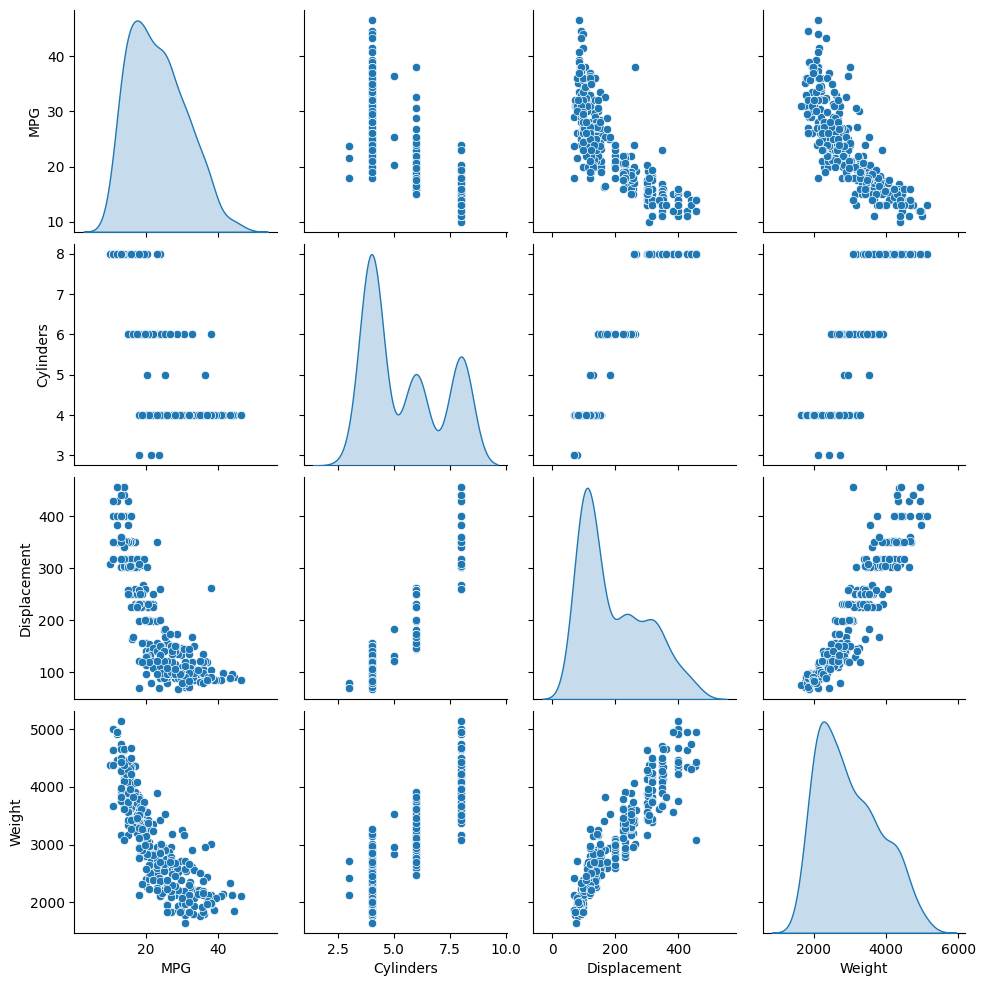
ตรวจสอบการกระจายร่วมของเสาสองสามคู่จากชุดการฝึก
แถวบนสุดแสดงให้เห็นว่าประสิทธิภาพการใช้เชื้อเพลิง (MPG) เป็นฟังก์ชันของพารามิเตอร์อื่นๆ ทั้งหมด แถวอื่น ๆ ระบุว่าเป็นหน้าที่ของกันและกัน
sns.pairplot(train_dataset[['MPG', 'Cylinders', 'Displacement', 'Weight']], diag_kind='kde')
<seaborn.axisgrid.PairGrid at 0x7f6bfdae9850>
ลองตรวจสอบสถิติโดยรวมด้วย โปรดทราบว่าคุณลักษณะแต่ละอย่างครอบคลุมช่วงที่แตกต่างกันมาก:
train_dataset.describe().transpose()
แยกคุณสมบัติออกจากป้ายกำกับ
แยกค่าเป้าหมาย—"ป้ายกำกับ"—ออกจากคุณสมบัติ ป้ายกำกับนี้เป็นค่าที่คุณจะฝึกให้โมเดลคาดการณ์
train_features = train_dataset.copy()
test_features = test_dataset.copy()

train_labels = train_features.pop('MPG')
test_labels = test_features.pop('MPG')
การทำให้เป็นมาตรฐาน
ในตารางสถิติ จะเห็นว่าช่วงของแต่ละฟีเจอร์แตกต่างกันอย่างไร:
train_dataset.describe().transpose()[['mean', 'std']]
แนวทางปฏิบัติที่ดีในการทำให้คุณลักษณะปกติที่ใช้มาตราส่วนและช่วงต่างๆ ต่างกัน ถือเป็นแนวทางปฏิบัติที่ดี
เหตุผลหนึ่งที่สำคัญคือเนื่องจากคุณลักษณะต่างๆ คูณด้วยน้ำหนักของรุ่น ดังนั้น ขนาดของเอาต์พุตและสเกลของการไล่ระดับสีจะได้รับผลกระทบจากสเกลของอินพุต
แม้ว่าแบบจำลอง อาจ มาบรรจบกันโดยไม่มีการทำให้เป็นมาตรฐานของคุณลักษณะ แต่การทำให้เป็นมาตรฐานทำให้การฝึกมีเสถียรภาพมากขึ้น
ชั้น Normalization
tf.keras.layers.Normalization เป็นวิธีที่ง่ายและสะอาดในการเพิ่มการทำให้เป็นมาตรฐานของคุณลักษณะในแบบจำลองของคุณ
ขั้นตอนแรกคือการสร้างเลเยอร์:
normalizer = tf.keras.layers.Normalization(axis=-1)
จากนั้น ปรับสถานะของเลเยอร์การประมวลผลล่วงหน้ากับข้อมูลโดยเรียก Normalization.adapt :
normalizer.adapt(np.array(train_features))
คำนวณค่าเฉลี่ยและความแปรปรวน และเก็บไว้ในเลเยอร์:
print(normalizer.mean.numpy())
[[   5.478  195.318  104.869 2990.252   15.559   75.898    0.178    0.197
     0.624]]
เมื่อเลเยอร์ถูกเรียก มันจะส่งคืนข้อมูลที่ป้อน โดยแต่ละฟีเจอร์จะถูกทำให้เป็นมาตรฐานโดยอิสระ:
first = np.array(train_features[:1])

with np.printoptions(precision=2, suppress=True):
  print('First example:', first)
  print()
  print('Normalized:', normalizer(first).numpy())
First example: [[   4.    90.    75.  2125.    14.5   74.     0.     0.     1. ]]

Normalized: [[-0.87 -1.01 -0.79 -1.03 -0.38 -0.52 -0.47 -0.5   0.78]]
การถดถอยเชิงเส้น
ก่อนสร้างแบบจำลองโครงข่ายประสาทลึก ให้เริ่มด้วยการถดถอยเชิงเส้นโดยใช้ตัวแปรหนึ่งตัวและหลายตัว
การถดถอยเชิงเส้นกับตัวแปรเดียว
เริ่มต้นด้วยการถดถอยเชิงเส้นตัวแปรเดียวเพื่อทำนาย 'MPG' จาก 'Horsepower'
การฝึกโมเดลด้วย tf.keras มักจะเริ่มต้นด้วยการกำหนดสถาปัตยกรรมโมเดล ใช้โมเดล tf.keras.Sequential ซึ่ง แสดงถึงลำดับของขั้นตอน
มีสองขั้นตอนในตัวแบบการถดถอยเชิงเส้นแบบตัวแปรเดียวของคุณ:
- ปรับคุณสมบัติอินพุต
'Horsepower'ให้เป็นมาตรฐานโดยใช้เลเยอร์การประมวลผลล่วงหน้าtf.keras.layers.Normalization - ใช้การแปลงเชิงเส้น (\(y = mx+b\)) เพื่อสร้าง 1 เอาต์พุตโดยใช้เลเยอร์เชิงเส้น (
tf.keras.layers.Dense)
จำนวน อินพุต สามารถกำหนดได้โดยอาร์กิวเมนต์ input_shape หรือโดยอัตโนมัติเมื่อรันโมเดลเป็นครั้งแรก
ขั้นแรก สร้างอาร์เรย์ NumPy ที่สร้างจากคุณสมบัติ 'Horsepower' จากนั้น ให้ยกตัวอย่าง tf.keras.layers.Normalization และปรับสถานะให้เข้ากับข้อมูล horsepower :
horsepower = np.array(train_features['Horsepower'])

horsepower_normalizer = layers.Normalization(input_shape=[1,], axis=None)
horsepower_normalizer.adapt(horsepower)
สร้างโมเดล Keras Sequential:
horsepower_model = tf.keras.Sequential([
    horsepower_normalizer,
    layers.Dense(units=1)
])

horsepower_model.summary()
Model: "sequential"
_________________________________________________________________
 Layer (type)                Output Shape              Param #
=================================================================
 normalization_1 (Normalizat  (None, 1)                3
 ion)

 dense (Dense)               (None, 1)                 2

=================================================================
Total params: 5
Trainable params: 2
Non-trainable params: 3
_________________________________________________________________
ตัวยึดตำแหน่ง32 โมเดลนี้จะทำนาย 'MPG' จาก 'Horsepower'
เรียกใช้โมเดลที่ไม่ได้รับการฝึกฝนในค่า 'แรงม้า' 10 ค่าแรก ผลลัพธ์จะออกมาไม่ดี แต่สังเกตว่ามันมีรูปร่างที่คาดไว้ (10, 1) :
horsepower_model.predict(horsepower[:10])
array([[-1.186],
       [-0.67 ],
       [ 2.189],
       [-1.662],
       [-1.504],
       [-0.59 ],
       [-1.782],
       [-1.504],
       [-0.392],
       [-0.67 ]], dtype=float32)
เมื่อสร้างโมเดลแล้ว ให้กำหนดค่าขั้นตอนการฝึกอบรมโดยใช้วิธี Keras Model.compile อาร์กิวเมนต์ที่สำคัญที่สุดในการรวบรวมคือการ loss และตัว optimizer เนื่องจากสิ่งเหล่านี้กำหนดสิ่งที่จะได้รับการปรับให้เหมาะสม ( mean_absolute_error ) และวิธี (โดยใช้ tf.keras.optimizers.Adam )
horsepower_model.compile(
    optimizer=tf.optimizers.Adam(learning_rate=0.1),
    loss='mean_absolute_error')
ใช้ Keras Model.fit เพื่อดำเนินการฝึกอบรม 100 ยุค:
%%time
history = horsepower_model.fit(
    train_features['Horsepower'],
    train_labels,
    epochs=100,
    # Suppress logging.
    verbose=0,
    # Calculate validation results on 20% of the training data.
    validation_split = 0.2)
CPU times: user 4.79 s, sys: 797 ms, total: 5.59 s
Wall time: 3.8 s
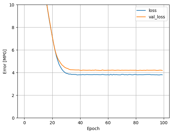
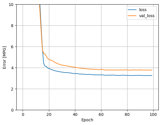
แสดงภาพความคืบหน้าการฝึกของโมเดลโดยใช้สถิติที่จัดเก็บไว้ในออบเจ็กต์ history :
hist = pd.DataFrame(history.history)
hist['epoch'] = history.epoch
hist.tail()
def plot_loss(history):
  plt.plot(history.history['loss'], label='loss')
  plt.plot(history.history['val_loss'], label='val_loss')
  plt.ylim([0, 10])
  plt.xlabel('Epoch')
  plt.ylabel('Error [MPG]')
  plt.legend()
  plt.grid(True)
plot_loss(history)
เก็บผลในชุดทดสอบในภายหลัง:
test_results = {}

test_results['horsepower_model'] = horsepower_model.evaluate(
    test_features['Horsepower'],
    test_labels, verbose=0)
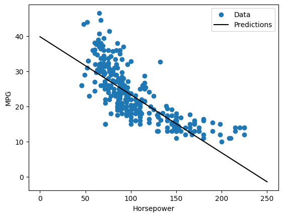
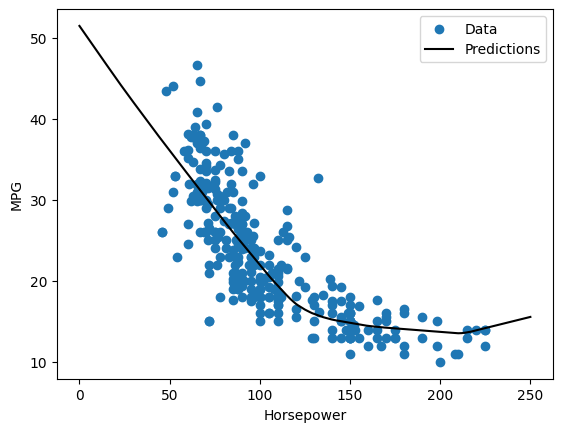
เนื่องจากนี่เป็นการถดถอยตัวแปรเดียว จึงง่ายต่อการดูการคาดการณ์ของแบบจำลองว่าเป็นฟังก์ชันของอินพุต:
x = tf.linspace(0.0, 250, 251)
y = horsepower_model.predict(x)
def plot_horsepower(x, y):
  plt.scatter(train_features['Horsepower'], train_labels, label='Data')
  plt.plot(x, y, color='k', label='Predictions')
  plt.xlabel('Horsepower')
  plt.ylabel('MPG')
  plt.legend()
plot_horsepower(x, y)
การถดถอยเชิงเส้นที่มีหลายอินพุต
คุณสามารถใช้การตั้งค่าที่เกือบจะเหมือนกันทั้งหมดเพื่อสร้างการคาดคะเนโดยอิงจากอินพุตหลายรายการ โมเดลนี้ยังคงใช้ \(y = mx+b\) เหมือนเดิม ยกเว้นว่า \(m\) เป็นเมทริกซ์ และ \(b\) เป็นเวกเตอร์
สร้างโมเดล Keras Sequential สองขั้นตอนอีกครั้งโดยที่เลเยอร์แรกเป็นแบบนอร์มัลไลเซอร์ ( normalizer tf.keras.layers.Normalization(axis=-1) ) ที่คุณกำหนดไว้ก่อนหน้านี้และปรับให้เข้ากับชุดข้อมูลทั้งหมด:
linear_model = tf.keras.Sequential([
    normalizer,
    layers.Dense(units=1)
])
เมื่อคุณเรียกใช้ Model.predict ในชุดอินพุต มันจะสร้างเอาต์พุต units=1 สำหรับแต่ละตัวอย่าง:
linear_model.predict(train_features[:10])
array([[ 0.441],
       [ 1.522],
       [ 0.188],
       [ 1.169],
       [ 0.058],
       [ 0.965],
       [ 0.034],
       [-0.674],
       [ 0.437],
       [-0.37 ]], dtype=float32)
เมื่อคุณเรียกใช้โมเดล เมทริกซ์น้ำหนักจะถูกสร้างขึ้น ตรวจสอบว่าน้ำหนัก kernel ( \(m\) ใน \(y=mx+b\)) มีรูปร่างเป็น (9, 1) :
linear_model.layers[1].kernel
<tf.Variable 'dense_1/kernel:0' shape=(9, 1) dtype=float32, numpy=
array([[-0.702],
       [ 0.307],
       [ 0.114],
       [ 0.233],
       [ 0.244],
       [ 0.322],
       [-0.725],
       [-0.151],
       [ 0.407]], dtype=float32)>
กำหนดค่าโมเดลด้วย Keras Model.compile และฝึกด้วย Model.fit สำหรับ 100 epochs:
linear_model.compile(
    optimizer=tf.optimizers.Adam(learning_rate=0.1),
    loss='mean_absolute_error')
%%time
history = linear_model.fit(
    train_features,
    train_labels,
    epochs=100,
    # Suppress logging.
    verbose=0,
    # Calculate validation results on 20% of the training data.
    validation_split = 0.2)
CPU times: user 4.89 s, sys: 740 ms, total: 5.63 s
Wall time: 3.75 s
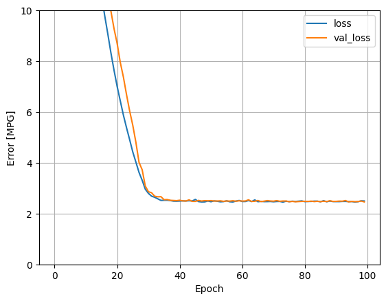
การใช้อินพุตทั้งหมดในโมเดลการถดถอยนี้ทำให้การฝึกอบรมและข้อผิดพลาดในการตรวจสอบต่ำกว่ามาก กว่า horsepower_model ซึ่งมีอินพุตเดียว:
plot_loss(history)
เก็บผลในชุดทดสอบในภายหลัง:
test_results['linear_model'] = linear_model.evaluate(
    test_features, test_labels, verbose=0)
การถดถอยด้วยโครงข่ายประสาทลึก (DNN)
ในส่วนก่อนหน้านี้ คุณได้ปรับใช้โมเดลเชิงเส้นสองแบบสำหรับอินพุตเดี่ยวและหลายอินพุต
ที่นี่ คุณจะใช้โมเดล DNN แบบอินพุตเดียวและหลายอินพุต
โดยพื้นฐานแล้วโค้ดจะเหมือนกัน ยกเว้นโมเดลถูกขยายเพื่อรวมเลเยอร์ที่ไม่ใช่เชิงเส้น "ที่ซ่อนอยู่" บางอัน ชื่อ "ซ่อน" ในที่นี้หมายความว่าไม่ได้เชื่อมต่อโดยตรงกับอินพุตหรือเอาต์พุต
โมเดลเหล่านี้จะมีเลเยอร์มากกว่าโมเดลเชิงเส้นเล็กน้อย:
- เลเยอร์การทำให้เป็น
normalizerเหมือนเมื่อก่อน (ด้วยhorsepower_normalizerสำหรับโมเดลอินพุตเดียวและนอร์มัลไลเซอร์สำหรับโมเดลหลายอินพุต) - เลเยอร์
Denseที่ไม่เป็นเชิงเส้นสองชั้นที่ซ่อนอยู่ด้วยฟังก์ชันการเปิดใช้งาน ReLU (relu) ที่ไม่เป็นเชิงเส้น - เลเยอร์เอาต์พุตเดี่ยวแบบเส้นตรง
Dense
ทั้งสองรุ่นจะใช้ขั้นตอนการฝึกอบรมเดียวกัน ดังนั้นวิธีการ compile จึงรวมอยู่ในฟังก์ชัน build_and_compile_model ด้านล่าง
def build_and_compile_model(norm):
  model = keras.Sequential([
      norm,
      layers.Dense(64, activation='relu'),
      layers.Dense(64, activation='relu'),
      layers.Dense(1)
  ])

  model.compile(loss='mean_absolute_error',
                optimizer=tf.keras.optimizers.Adam(0.001))
  return model
การถดถอยโดยใช้ DNN และอินพุตเดียว
สร้างโมเดล DNN ที่มีเพียง 'Horsepower' เป็นอินพุตและ horsepower_normalizer (กำหนดไว้ก่อนหน้านี้) เป็นเลเยอร์การทำให้เป็นมาตรฐาน:
dnn_horsepower_model = build_and_compile_model(horsepower_normalizer)
โมเดลนี้มีพารามิเตอร์ที่ฝึกได้ค่อนข้างน้อยกว่าโมเดลเชิงเส้น:
dnn_horsepower_model.summary()
Model: "sequential_2"
_________________________________________________________________
 Layer (type)                Output Shape              Param #
=================================================================
 normalization_1 (Normalizat  (None, 1)                3
 ion)

 dense_2 (Dense)             (None, 64)                128

 dense_3 (Dense)             (None, 64)                4160

 dense_4 (Dense)             (None, 1)                 65

=================================================================
Total params: 4,356
Trainable params: 4,353
Non-trainable params: 3
_________________________________________________________________
ฝึกโมเดลด้วย Keras Model.fit :
%%time
history = dnn_horsepower_model.fit(
    train_features['Horsepower'],
    train_labels,
    validation_split=0.2,
    verbose=0, epochs=100)
CPU times: user 5.07 s, sys: 691 ms, total: 5.76 s
Wall time: 3.92 s
ตัวยึดตำแหน่ง60
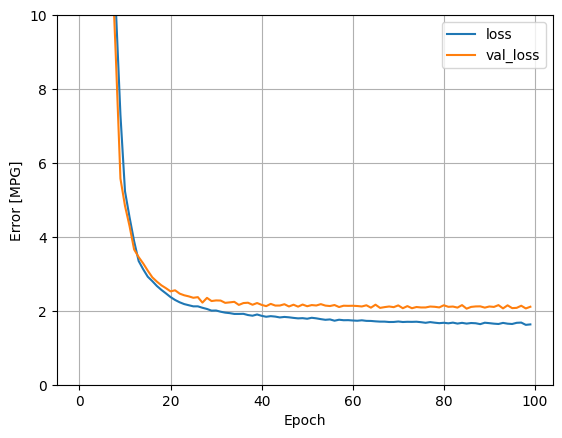
โมเดลนี้ทำได้ดีกว่า horsepower_model แบบ single-input แบบ single-input เล็กน้อย:
plot_loss(history)
หากคุณพล็อตการคาดคะเนเป็นฟังก์ชันของ 'Horsepower' คุณควรสังเกตว่าโมเดลนี้ใช้ประโยชน์จากความไม่เชิงเส้นของเลเยอร์ที่ซ่อนอยู่ได้อย่างไร:
x = tf.linspace(0.0, 250, 251)
y = dnn_horsepower_model.predict(x)
plot_horsepower(x, y)
เก็บผลในชุดทดสอบในภายหลัง:
test_results['dnn_horsepower_model'] = dnn_horsepower_model.evaluate(
    test_features['Horsepower'], test_labels,
    verbose=0)
การถดถอยโดยใช้ DNN และอินพุตหลายตัว
ทำซ้ำขั้นตอนก่อนหน้าโดยใช้อินพุตทั้งหมด ประสิทธิภาพของแบบจำลองดีขึ้นเล็กน้อยในชุดข้อมูลการตรวจสอบ
dnn_model = build_and_compile_model(normalizer)
dnn_model.summary()
Model: "sequential_3"
_________________________________________________________________
 Layer (type)                Output Shape              Param #
=================================================================
 normalization (Normalizatio  (None, 9)                19
 n)

 dense_5 (Dense)             (None, 64)                640

 dense_6 (Dense)             (None, 64)                4160

 dense_7 (Dense)             (None, 1)                 65

=================================================================
Total params: 4,884
Trainable params: 4,865
Non-trainable params: 19
_________________________________________________________________
%%time
history = dnn_model.fit(
    train_features,
    train_labels,
    validation_split=0.2,
    verbose=0, epochs=100)
CPU times: user 5.08 s, sys: 725 ms, total: 5.8 s
Wall time: 3.94 s
plot_loss(history)
เก็บผลในชุดทดสอบ:
test_results['dnn_model'] = dnn_model.evaluate(test_features, test_labels, verbose=0)
ประสิทธิภาพ
เนื่องจากทุกรุ่นได้รับการฝึกอบรม คุณสามารถตรวจสอบประสิทธิภาพของชุดทดสอบได้:
pd.DataFrame(test_results, index=['Mean absolute error [MPG]']).T
ผลลัพธ์เหล่านี้ตรงกับข้อผิดพลาดในการตรวจสอบที่สังเกตได้ระหว่างการฝึก
ทำนายฝัน
ตอนนี้คุณสามารถคาดการณ์ด้วย dnn_model ในชุดการทดสอบโดยใช้ Keras Model.predict และตรวจสอบการสูญเสีย:
test_predictions = dnn_model.predict(test_features).flatten()

a = plt.axes(aspect='equal')
plt.scatter(test_labels, test_predictions)
plt.xlabel('True Values [MPG]')
plt.ylabel('Predictions [MPG]')
lims = [0, 50]
plt.xlim(lims)
plt.ylim(lims)
_ = plt.plot(lims, lims)

ดูเหมือนว่าโมเดลคาดการณ์ได้ดีพอสมควร
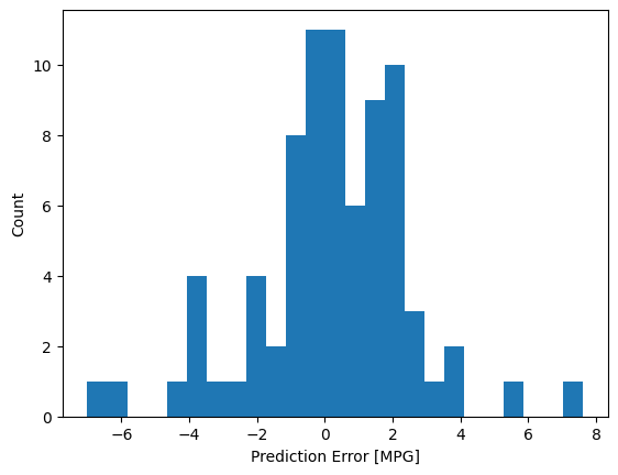
ตอนนี้ ตรวจสอบการกระจายข้อผิดพลาด:
error = test_predictions - test_labels
plt.hist(error, bins=25)
plt.xlabel('Prediction Error [MPG]')
_ = plt.ylabel('Count')
หากคุณพอใจกับโมเดลนี้ ให้บันทึกไว้เพื่อใช้ในภายหลังด้วย Model.save :
dnn_model.save('dnn_model')
2022-01-26 07:26:13.372245: W tensorflow/python/util/util.cc:368] Sets are not currently considered sequences, but this may change in the future, so consider avoiding using them.
INFO:tensorflow:Assets written to: dnn_model/assets
หากคุณรีโหลดโมเดล มันจะให้ผลลัพธ์ที่เหมือนกัน:
reloaded = tf.keras.models.load_model('dnn_model')

test_results['reloaded'] = reloaded.evaluate(
    test_features, test_labels, verbose=0)
pd.DataFrame(test_results, index=['Mean absolute error [MPG]']).T
บทสรุป
สมุดบันทึกนี้แนะนำเทคนิคบางประการเพื่อจัดการกับปัญหาการถดถอย ต่อไปนี้เป็นเคล็ดลับเพิ่มเติมที่อาจช่วยได้:
- ข้อผิดพลาดกำลังสองเฉลี่ย (MSE) (
tf.losses.MeanSquaredError) และข้อผิดพลาดแบบสัมบูรณ์เฉลี่ย (MAE) (tf.losses.MeanAbsoluteError) เป็นฟังก์ชันการสูญเสียทั่วไปที่ใช้สำหรับปัญหาการถดถอย MAE มีความไวต่อค่าผิดปกติน้อยกว่า ฟังก์ชันการสูญเสียต่างๆ ใช้สำหรับปัญหาการจำแนกประเภท - ในทำนองเดียวกัน ตัวชี้วัดการประเมินที่ใช้สำหรับการถดถอยแตกต่างจากการจัดประเภท
- เมื่อคุณลักษณะข้อมูลป้อนที่เป็นตัวเลขมีค่าที่มีช่วงต่างกัน คุณลักษณะแต่ละรายการควรได้รับการปรับขนาดอย่างอิสระเพื่อให้อยู่ในช่วงเดียวกัน
- Overfitting เป็นปัญหาทั่วไปสำหรับโมเดล DNN แม้ว่าจะไม่ใช่ปัญหาสำหรับบทช่วยสอนนี้ ไปที่บทแนะนำ Overfit และ underfit เพื่อรับความช่วยเหลือเพิ่มเติมเกี่ยวกับเรื่องนี้
# MIT License
#
# Copyright (c) 2017 François Chollet
#
# Permission is hereby granted, free of charge, to any person obtaining a
# copy of this software and associated documentation files (the "Software"),
# to deal in the Software without restriction, including without limitation
# the rights to use, copy, modify, merge, publish, distribute, sublicense,
# and/or sell copies of the Software, and to permit persons to whom the
# Software is furnished to do so, subject to the following conditions:
#
# The above copyright notice and this permission notice shall be included in
# all copies or substantial portions of the Software.
#
# THE SOFTWARE IS PROVIDED "AS IS", WITHOUT WARRANTY OF ANY KIND, EXPRESS OR
# IMPLIED, INCLUDING BUT NOT LIMITED TO THE WARRANTIES OF MERCHANTABILITY,
# FITNESS FOR A PARTICULAR PURPOSE AND NONINFRINGEMENT. IN NO EVENT SHALL
# THE AUTHORS OR COPYRIGHT HOLDERS BE LIABLE FOR ANY CLAIM, DAMAGES OR OTHER
# LIABILITY, WHETHER IN AN ACTION OF CONTRACT, TORT OR OTHERWISE, ARISING
# FROM, OUT OF OR IN CONNECTION WITH THE SOFTWARE OR THE USE OR OTHER
# DEALINGS IN THE SOFTWARE.